Transforming Functions with Purpose

A transformation changes where or how a familiar function appears without requiring every graph to be rebuilt point by point. The notation is compact, but its compactness can hide the mechanism. Changes outside a function act on outputs, while changes inside act on the inputs delivered to the function. That distinction explains both the order and the apparently reversed sign of horizontal shifts. This lesson develops transformation rules from coordinate reasoning rather than memorized slogans.

The guiding question is how a symbolic change moves individual points of a graph. We will begin from landmarks such as intercepts, vertices, endpoints, and asymptotes. We will then derive vertical and horizontal effects, including reflections and stretches. Finally, we will compose several transformations while preserving a clear order of reasoning. Each result should be predictable before graphing software is consulted.

By the end, you should map points from $y=f(x)$ to a transformed graph, explain why $f(x-h)$ moves right, and distinguish vertical from horizontal scaling. You should identify which geometric features remain invariant. You should also diagnose common sign and order errors. The next lesson uses this machinery to compare parameters across polynomial, exponential, logarithmic, and trigonometric families.

Begin with landmarks and invariants

A parent function is a convenient reference member of a family, not an ancestor with special mathematical authority. For $f(x)=x^2$, the vertex $(0,0)$ is a landmark, the vertical axis is an axis of symmetry, and the range begins at zero. For $f(x)=|x|$, the corner at the origin is a landmark. For $f(x)=\sqrt{x}$, the origin is a domain endpoint. Tracking landmarks makes a transformation visible with fewer calculations.

An invariant is a feature preserved by a particular transformation. A translation preserves distances, orientation, and overall shape. A nonzero vertical stretch preserves input locations of zeros but changes most output distances. A reflection reverses orientation while preserving distance from the reflecting axis. Identifying invariants lets us check a graph after it is drawn. A transformed picture that violates an expected invariant contains an error.

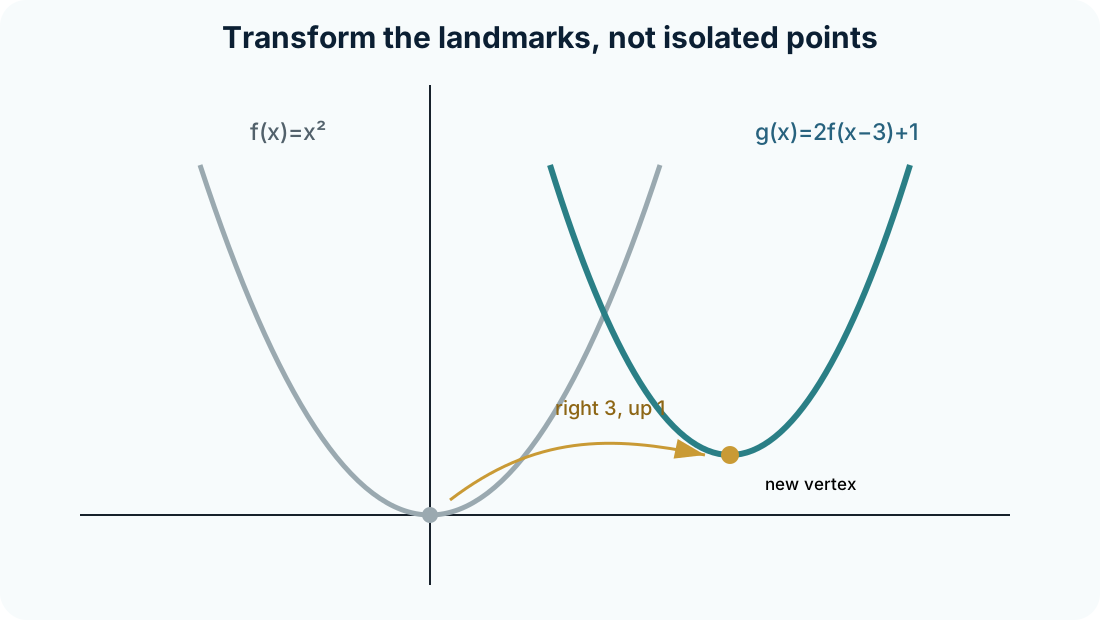
Use a small point set as an anchor. The points $(-1,1)$, $(0,0)$, and $(1,1)$ lie on $y=x^2$. Rather than generating dozens of values for every transformation, map these points and the vertex. Then use the known family shape to complete the sketch. This is efficient because the reasoning operates on the function as an object.

Outside changes act on outputs

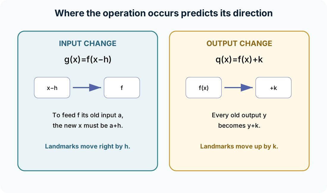
For $g(x)=f(x)+k$, the input sent into $f$ is unchanged and $k$ is added afterward. Every point $(x,y)$ on $f$ becomes $(x,y+k)$ on $g$. Positive $k$ shifts the graph upward, and negative $k$ shifts it downward. Domain inputs remain unchanged, while the range translates vertically. Vertical motion follows the visible sign because the operation acts directly on outputs.

For $g(x)=af(x)$, every output is multiplied by $a$. When $|a|>1$, vertical distances from the horizontal axis grow; when $0<|a|<1$, they shrink. If $a<0$, output signs reverse and the graph reflects across the horizontal axis. A zero of $f$ remains a zero because $a\cdot0=0$. Multiplication therefore changes height without moving the input where a landmark occurs.

Units clarify what these constants mean. If $f(t)$ is a temperature in degrees Celsius, then $k$ must also carry degrees Celsius for $f(t)+k$ to be valid. The factor $a$ is dimensionless when it merely rescales the same output quantity. A context may make negative scaling nonsensical even though the graph operation is algebraically legal. Symbolic possibility and model suitability must be distinguished.

Inside changes act on inputs

For $g(x)=f(x-h)$, the function receives input $x-h$. To reproduce the old output $f(u)$, we require $x-h=u$, so $x=u+h$. Thus each point $(u,f(u))$ moves to $(u+h,f(u))$. Positive $h$ shifts the graph right. The sign appears reversed only when the expression is read as an instruction to the visible coordinate rather than as an input equation.

For $g(x)=f(bx)$, the old input $u$ is reproduced when $bx=u$, giving $x=\frac{u}{b}$. Horizontal coordinates are divided by $b$. If $|b|>1$, the graph is compressed horizontally; if $0<|b|<1$, it stretches. A negative $b$ also reflects the graph across the vertical axis. The reciprocal effect follows from solving for the new input location.

Domains must transform with the inputs. If $f$ is defined for $u\ge0$, then $f(x-3)$ requires $x-3\ge0$, or $x\ge3$. If $f$ has a vertical asymptote where its input equals zero, then $f(x+2)$ places that condition at $x=-2$. These are not extra rules. They are consequences of asking which visible inputs produce allowed internal inputs.

Compose transformations in a controlled order

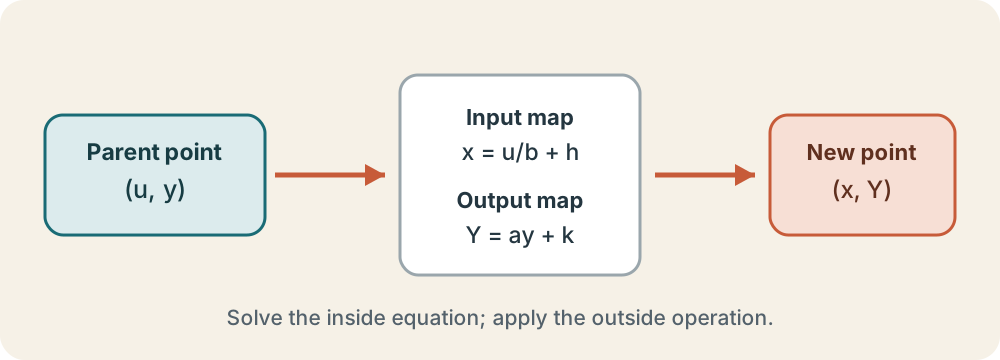
Consider $g(x)=-2f(3(x-4))+5$. Start with a parent point $(u,y)$, where $y=f(u)$. The internal equation $3(x-4)=u$ gives $x=\frac{u}{3}+4$. The outside operations give the new output $-2y+5$. Thus the coordinate map is $(u,y)\mapsto\left(\frac{u}{3}+4,-2y+5\right)$. This single map prevents conflicting verbal orders.

The graph is compressed horizontally by a factor of $\frac13$, shifted right four units, reflected across the horizontal axis, stretched vertically by two, and shifted up five. Some operations commute and some do not. Multiplying outputs before adding five differs from multiplying the already shifted outputs. Parentheses and the coordinate map make the intended structure explicit. A sketch should be checked against at least three mapped landmarks.

Graphing software is useful for verification after a prediction has been made. Enter the parent and transformed functions together and compare corresponding landmarks. If the predicted shift is reversed, return to the input equation rather than memorizing a correction. If the vertical location is wrong, check the order of multiplication and addition. The tool should test reasoning, not replace it.

Synthesis and transition

Take $f(x)=|x|$ and analyze $g(x)=-\frac12|2(x+3)|+4$. Write the coordinate map, transform the corner and two symmetric points, and state the new domain and range. Describe each transformation in words and identify one invariant. Then sketch before checking electronically. Explain any discrepancy using the symbolic structure.

Next create two different formulas that move the parabola $y=x^2$ to a vertex at $(2,-3)$ but give different widths. Map the points $(-1,1)$, $(0,0)$, and $(1,1)$ for each formula. Explain which parameter controls the shared location and which controls the difference. Your explanation should connect symbols, coordinates, and visible shape. Do not rely on “inside is opposite” as the entire justification.

A transformation is a rule for relocating and rescaling the points of a function. Outside operations act on outputs directly, while inside operations determine which visible input reproduces an old input. Coordinate maps unify shifts, stretches, and reflections and provide a reliable error check. With that mechanism established, the next lesson compares how meaningful parameters behave across several major function families. The emphasis will shift from moving one graph to interpreting families of related models.