Making Approaches Precise: Epsilon and Delta

Earlier lessons said that outputs can be made as close to a destination as desired by choosing inputs sufficiently close to a target. Epsilon-delta language makes every part of that sentence measurable. Epsilon names the permitted output error. Delta names an input radius that is small enough to guarantee that error. The definition does not create a new kind of limit; it states the familiar nearby-control claim without relying on a picture or a sample table.

This lesson translates the definition, develops a proof workflow, and proves a simple linear limit. We will also explain why delta may depend on epsilon and why the center input is excluded. The guiding question is: how can an input tolerance guarantee an output tolerance for every allowed nearby input? The next lesson turns from finite output destinations to unbounded behavior and far-away inputs.

By the end, you should read the formal definition in words, distinguish epsilon from delta, construct a valid delta choice for a linear function, and verify the implication chain. You should recognize that guessing a delta is not enough unless the inequality proof works. You should also interpret the definition as a tolerance-design problem. Formal language should clarify the geometry rather than obscure it.

Read the definition as a conditional guarantee

The statement

$$\lim_{x\to a}f(x)=L$$

means that for every $\varepsilon>0$, there exists a $\delta>0$ such that

$$0<|x-a|<\delta \quad\Longrightarrow\quad |f(x)-L|<\varepsilon.$$

The phrase “for every” makes epsilon a challenge supplied by the reader. The phrase “there exists” permits us to choose a delta tailored to that challenge.

The input condition $0<|x-a|<\delta$ describes a punctured delta-neighborhood. The output conclusion $|f(x)-L|<\varepsilon$ describes an epsilon-neighborhood around the limiting value. The implication says that every allowed input close enough to $a$ produces an output close enough to $L$. The center is excluded because the limit concerns nearby behavior rather than requiring $f(a)$ to exist.

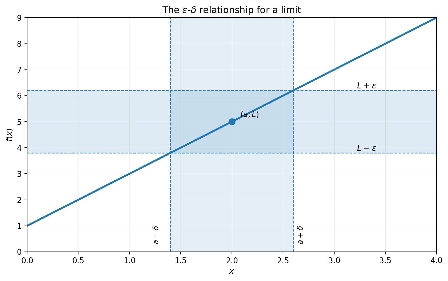
Epsilon and delta do not play symmetric roles. Epsilon is specified first as the desired output accuracy. Delta is selected in response after examining how the function turns input error into output error. A smaller epsilon may require a smaller delta. The definition guarantees a strategy for every positive requested tolerance, not one fixed radius for all requests.

Turn geometry into an inequality chain

To prove $\lim_{x\to2}(3x+1)=7$, begin with the output error:

$$|(3x+1)-7|=|3x-6|=3|x-2|.$$

To make this less than epsilon, it is sufficient to require $|x-2|<\frac{\varepsilon}{3}$. Choose $\delta=\frac{\varepsilon}{3}$. The choice comes from solving the output-error inequality backward.

The forward proof begins by assuming $0<|x-2|<\delta$. Then

$$|(3x+1)-7|=3|x-2|<3\delta =3\left(\frac{\varepsilon}{3}\right)=\varepsilon.$$

The final strict inequality establishes the required conclusion. Every line connects the input condition to the requested output bound.

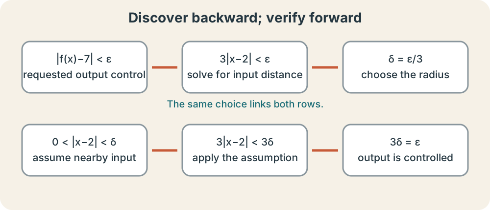
The order is strategic. Working backward discovers a sufficient delta choice; working forward proves that the choice succeeds. Writing only $\delta=\frac\varepsilon3$ does not explain why it works. Writing a chain that ends in a number unrelated to epsilon does not meet the definition. A valid proof controls the exact output-error expression.

Delta may depend on epsilon

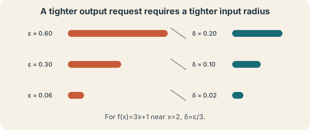
For the linear example, halving epsilon halves delta. This dependence is expected. Asking outputs to lie within $0.01$ of seven is more demanding than asking them to lie within one unit of seven. The allowed input radius must respond to the requested precision. Delta is a rule or choice, not a universal constant unrelated to the challenge.

Suppose epsilon is $0.06$ output units. The choice $\delta=\frac{0.06}{3}=0.02$ input units works for the function $3x+1$ near two. If the input lies within $0.02$ of two, the output lies within $0.06$ of seven. This is a quantitative local-error statement. Units should be attached in applied models, because epsilon and delta generally measure different quantities.

For a position model, delta might be seconds while epsilon is meters. The relation between them is determined by local behavior, such as a rate bound. A bare statement that “delta equals epsilon” may work for some special functions but carries no general meaning. The function mediates between input and output spaces. This is why the proof begins by analyzing $|f(x)-L|$.

Bounded factors require an auxiliary restriction

Nonlinear proofs often produce a product containing both $|x-a|$ and another changing factor. For $x^2$ near two,

$$|x^2-4|=|x-2||x+2|.$$

The first factor is controlled by delta, but $|x+2|$ also needs a bound. Impose an auxiliary condition such as $|x-2|<1$. Then $1<x<3$, so $3<x+2<5$ and $|x+2|<5$.

Choose $\delta=\min\left(1,\frac{\varepsilon}{5}\right)$. If $0<|x-2|<\delta$, both the auxiliary bound and the epsilon-driven bound hold. Therefore

$$|x^2-4|=|x-2||x+2|<5|x-2|<5\delta\le\varepsilon.$$

The minimum combines two requirements into one permitted input radius.

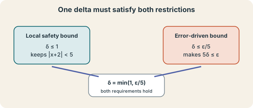
The auxiliary restriction is not a trick added after failure. It reflects local reasoning: near two, the factor $x+2$ cannot grow without bound. The proof makes “near” numerically useful by turning it into a bounded interval. Similar bounding steps appear throughout analysis. They provide the bridge from algebraic factorization to controlled error.

Common misconceptions

The definition does not say choose one delta that works for all epsilon. It says every requested positive epsilon must have some positive responding delta. It does not permit delta equal to zero, because an input neighborhood must contain nearby points. It does not require evaluating $f(a)$. The punctured condition protects the distinction between limit and point value.

Epsilon is not automatically a small decimal chosen by the author. It is arbitrary and positive. A proof must work for $\varepsilon=1$, $\varepsilon=10^{-6}$, and every other positive tolerance. Demonstrating several sample epsilons can build intuition but does not prove the universal claim. The symbolic choice of delta is what covers all cases.

Graphs are helpful but not decisive. A diagram can show nested horizontal and vertical bands, but it cannot certify every input in the band. The inequality proof supplies that guarantee. Conversely, a proof should remain connected to the geometry it formalizes. Epsilon measures vertical output distance; delta measures horizontal input distance. Reading symbols spatially reduces notation errors.

Synthesis and transition

Prove $\lim_{x\to4}(2x-1)=7$ using the formal definition. Begin by simplifying the output error, choose delta in terms of epsilon, and then write the implication proof forward. State which quantity is input distance and which is output distance. If $x$ is measured in seconds and the function output in meters, annotate the dimensions of delta and epsilon.

Then prove $\lim_{x\to1}x^2=1$ using an auxiliary bound. Explain why $|x+1|$ cannot simply be replaced by two at nearby inputs. Choose a suitable local radius, combine it with the epsilon-driven bound using a minimum, and verify the chain. Compare this proof with the linear case to identify why nonlinear structure needs one extra step.

Epsilon-delta language formalizes the nearby-control idea already present in every finite limit. Epsilon specifies output accuracy, delta supplies sufficient input closeness, and the proof links them for every allowed nearby input. Linear functions reveal the basic workflow, while nonlinear factors require local bounds. The next lesson studies behavior that does not approach a finite output value: vertical asymptotes and limits at infinity. The same emphasis on controlled behavior remains, but the destination language changes.