Difference Quotients as Movable Secants

An average rate normally uses two fixed endpoints. Calculus needs a way to keep one endpoint fixed while allowing the other to move. The difference quotient performs that job. It is not yet a derivative and it does not permit a zero interval. It is a symbolic family of ordinary secant slopes indexed by a nonzero displacement.

This lesson develops the $x+h$ and $x-a$ forms from the endpoint formula. We will simplify quotients without illegal cancellation, interpret the remaining variable, and connect algebra to moving secant lines. We will also preserve units in physical examples. The guiding question is: how can one expression represent many nearby average rates? Limits will later ask whether those rates approach a common value.

By the end, you should construct both common difference-quotient forms, simplify polynomial and rational examples, and state all restrictions. You should explain why $h=0$ remains excluded after cancellation. You should interpret $h$ as a signed input displacement. You should connect each algebraic term to a secant interval. You should also identify when directional values disagree.

Derive the x-plus-h form

Start with average rate from input $x$ to input $x+h$. The input change is $(x+h)-x=h$. The output change is $f(x+h)-f(x)$. Therefore the secant slope is

$$\frac{f(x+h)-f(x)}{h},\qquad h\ne0.$$

The condition $h\ne0$ is part of the expression’s meaning because the endpoints must be distinct.

The letter $h$ is a signed displacement, not necessarily a small positive number. Positive $h$ places the second endpoint to the right of $x$, while negative $h$ places it to the left. Its magnitude is the interval width. Holding $x$ fixed and varying $h$ generates a family of secant lines. Later, $h\to0$ will describe shrinking intervals without ever substituting zero into the quotient.

Function notation must be handled before expansion. If $f(x)=3x^2-2x+5$, then $f(x+h)=3(x+h)^2-2(x+h)+5$. Replacing only selected occurrences of $x$ corrupts the input substitution. Parentheses show that the entire input is $x+h$. Careful substitution prevents errors that no later algebra can repair.

Simplify without erasing restrictions

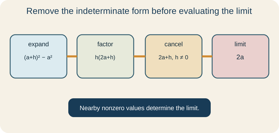
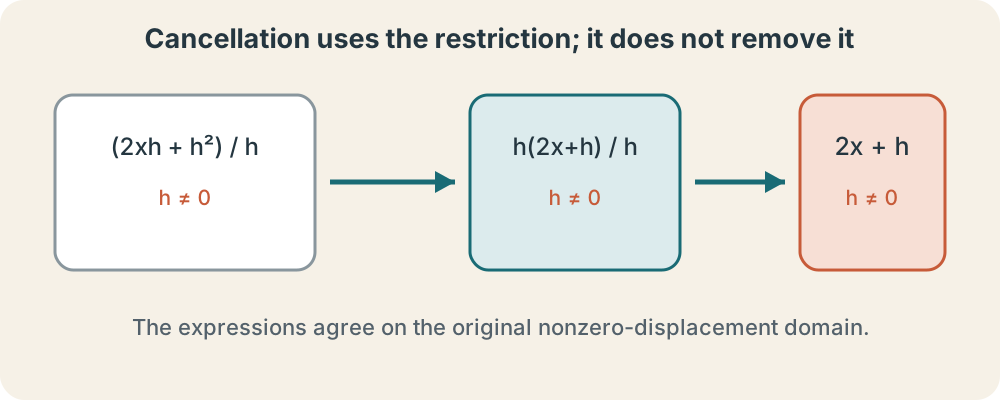
For $f(x)=x^2$, the quotient becomes

$$\frac{(x+h)^2-x^2}{h} =\frac{2xh+h^2}{h} =2x+h,\qquad h\ne0.$$

The factor $h$ cancels because it is nonzero on the quotient’s domain. Cancellation does not make the original quotient defined at $h=0$. It creates a simpler expression equal to the original at every allowed nonzero $h$.

For $f(x)=\frac1x$, additional restrictions appear. The quotient is

$$\frac{\frac1{x+h}-\frac1x}{h} =\frac{-1}{x(x+h)},$$

provided $h\ne0$, $x\ne0$, and $x+h\ne0$. Combining the inner fractions requires the common denominator $x(x+h)$. Every original restriction survives simplification. A compact final expression must not conceal inputs that were never legal.

The simplification goal is structural rather than cosmetic. Terms should be arranged so the displacement factor becomes visible. Factoring, expanding, rationalizing, or combining fractions may be appropriate depending on the function. Cancelling individual terms across addition is never valid. Each transformation must preserve equality on the stated restricted domain.

Use a fixed target instead

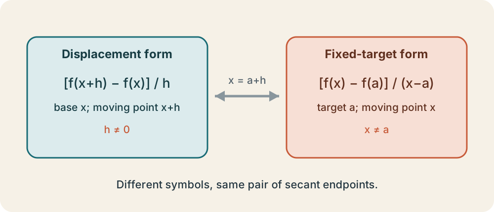
Sometimes a particular target input $a$ is more useful than a generic input $x$. Comparing $f(x)$ with $f(a)$ gives

$$\frac{f(x)-f(a)}{x-a},\qquad x\ne a.$$

Here $x$ is the moving endpoint and $a$ is fixed. Setting $x=a+h$ converts this expression into the $h$ form. The two notations describe the same secant geometry with different variables.

For $f(x)=x^2$ at $a=3$, the quotient is

$$\frac{x^2-9}{x-3}=x+3,\qquad x\ne3.$$

The simplified expression reveals nearby slopes, but the original quotient remains undefined at the target. Values from both sides approach $6$ as $x$ approaches $3$. This is evidence for a local slope that will later be defined using a limit.

Choose the form that matches the question. The $h$ form emphasizes displacement from a variable base input and is convenient for deriving derivative formulas. The $x-a$ form emphasizes behavior near one fixed target and aligns closely with limit notation. Neither is more correct. Translating between them should preserve the endpoints and restrictions.

Connect algebra to movable secants

For $f(x)=x^2$ at base input $x=1$, the simplified $h$ quotient is $2+h$. When $h=1$, the secant slope is $3$. When $h=0.5$, it is $2.5$. When $h=-0.5$, it is $1.5$. The slopes change because the parabola is nonlinear, yet they organize around a common local value near $2$.

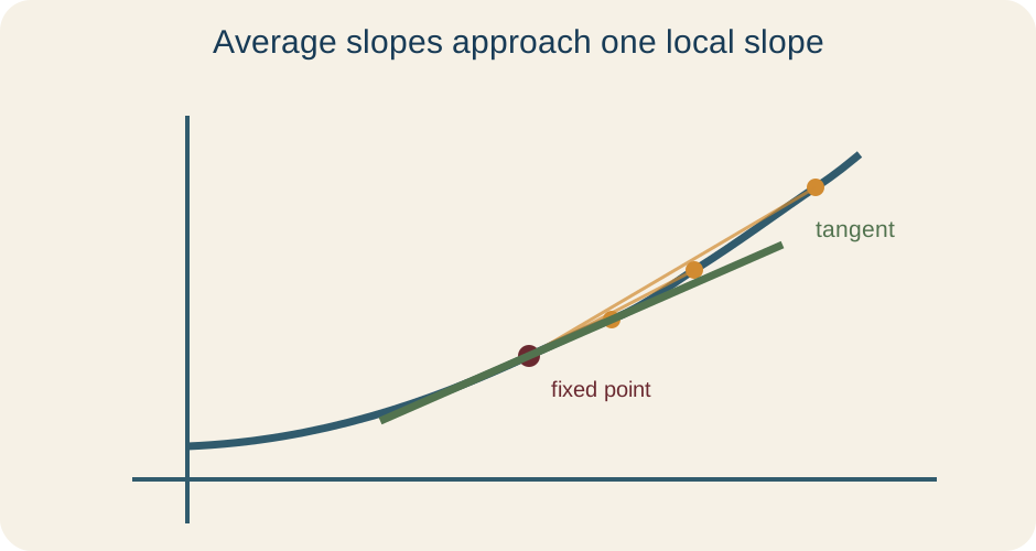
The graph and algebra report the same structure. Smaller positive displacements rotate right-side secants toward one line, while smaller negative displacements rotate left-side secants toward it from the other direction. A table can display numerical stabilization. No single representation proves the conclusion by itself at this stage. Their agreement motivates the limit question.

For $f(x)=|x|$ at $x=0$, the quotient is $\frac{|h|}{h}$. It equals $1$ for positive $h$ and $-1$ for negative $h$. Both directional families are stable, but they disagree. This counterexample shows why shrinking an interval does not guarantee one local slope. Directional agreement must be examined.

Units and interpretation

Let position be $s(t)=5t^2-3t$ meters with time in seconds. The quotient from $t$ to $t+h$ has units

$$\frac{s(t+h)-s(t)}{h} \quad\text{in}\quad \frac{\mathrm{m}}{\mathrm{s}}.$$

The symbol $h$ carries seconds, not merely a dimensionless number. Simplification changes the formula but not its physical dimension.

The sign of $h$ identifies whether the second time lies after or before the base time. The sign of the quotient describes average velocity, which may differ from the sign of $h$. A negative displacement and negative position change produce a positive quotient. Tracking units and signs separately prevents verbal confusion. The algebra should be interpreted only after the ordered interval is clear.

Measurement data introduce uncertainty. Subtracting nearby positions can yield a small numerator dominated by instrument resolution. Dividing by a very small time interval may amplify that uncertainty. The ideal limit can still define a model’s instantaneous velocity, but an experiment estimates it imperfectly. Calculus supplies a target, not immunity from measurement error.

Synthesis and transition

For $f(x)=2x^2-5x+1$, construct and simplify $\frac{f(x+h)-f(x)}{h}$. State $h\ne0$ on every equivalent line where it matters. Evaluate the simplified result at $x=3$ for $h=1$, $0.1$, $-0.1$, and $-1$. Describe the secant intervals and explain the visible stabilization. Attach no physical units because this example is abstract.

Then let $s(t)=4t^2+2t$ meters and repeat at $t=2\,\mathrm{s}$. Attach $\frac{\mathrm{m}}{\mathrm{s}}$ to every computed rate. Explain what positive and negative $h$ mean and why $h=0$ remains forbidden. Compare the table, symbolic expression, and imagined secant lines. Identify which representation makes each conclusion easiest to see.

A difference quotient is a movable secant slope, not an instruction to divide by zero. Its algebra preserves endpoint order, domain restrictions, and units. Simplification reveals how average rates depend on displacement and base location. The next lesson strengthens the algebraic tools needed to restructure quotients reliably. After that preparation, limits will turn the observed approach of secant slopes into a precise mathematical object.