Continuity and the Intermediate Value Theorem

A function is continuous at a point when its nearby behavior and its assigned point value tell one consistent story. Informal language calls this a graph that can be drawn without lifting a pencil, but that picture can hide the actual test. A graph can be drawn in one stroke across a wide interval while still failing at a single carefully assigned point. Calculus needs a definition that detects that local failure. Continuity supplies that definition and then turns it into a powerful existence guarantee.

This lesson asks two related questions. First, how do we decide whether a function is continuous at a particular input? Second, what can continuity guarantee even when we cannot solve an equation exactly? We will distinguish holes, jumps, and unbounded breaks; then we will use the Intermediate Value Theorem, abbreviated IVT, to prove that a target output must be reached. The essential idea is that a continuous function cannot teleport from one height to another while skipping every height in between.

By the end, you should be able to apply the three-part continuity test, classify common discontinuities, and state every hypothesis of the IVT before using it. You should also recognize the difference between proving that a solution exists and finding its exact numerical value. This closes the limits unit. The derivative unit will use continuity as a background condition while returning to the local-rate question that originally motivated limits.

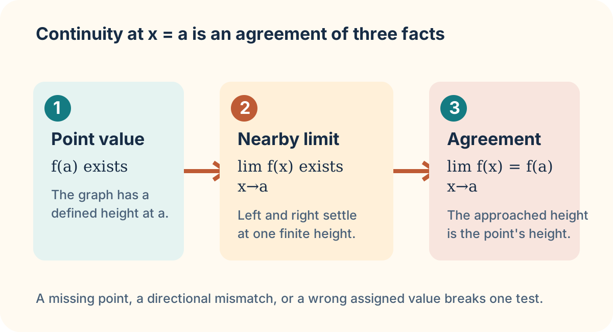
The three facts that must agree

The compact definition is

$$\lim_{x\to a}f(x)=f(a).$$

The left side concerns values of $f(x)$ for inputs near $a$, while the right side is the value assigned at exactly $a$. For this equation even to make sense, the point value $f(a)$ must exist and the two-sided limit must exist. Finally, those two finite values must agree. Continuity is therefore not just a limit condition and not just a point-value condition.

For a polynomial such as $p(x)=x^3-4x+1$, each ordinary substitution is valid, and the nearby outputs approach the substituted output. Thus polynomials are continuous at every real input. Rational functions are continuous wherever their denominators are nonzero. Trigonometric, exponential, and logarithmic functions are continuous on their respective domains. These facts are useful, but their domain restrictions still matter: a familiar formula does not become continuous at an input where it is undefined.

Consider the piecewise function $f(x)=x+2$ for $x\ne1$ and $f(1)=10$. As $x$ approaches one, the expression $x+2$ approaches three. The point value exists, but it is ten rather than three. The limit and the point value disagree, so $f$ is not continuous at one. Redefining $f(1)=3$ would repair the function at that point; this is a removable discontinuity.

Diagnose the kind of break

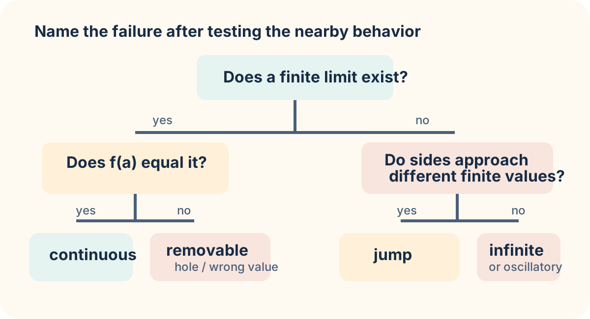
A removable discontinuity occurs when a finite two-sided limit exists but the function is missing there or has been assigned the wrong value. Factoring often exposes this case. The expression $\frac{x^2-9}{x-3}$ simplifies to $x+3$ for $x\ne3$, so its nearby limit at three is six, but the original expression has no value at three. A single assigned value of six would make the extended function continuous. The hole is a local bookkeeping problem, not a failure of nearby agreement.

A jump discontinuity occurs when the left- and right-hand limits are finite but unequal. A step model that changes from a shipping cost of $5\,\mathrm{USD}$ to $8\,\mathrm{USD}$ at a mass threshold has a jump if the threshold rule assigns one of those values. No one point value can repair a jump because the nearby behavior itself does not settle on one number. The issue is not a missing dot; it is incompatible directional evidence. Always compute the directional limits before labeling a break removable.

An infinite discontinuity occurs when outputs become unbounded near the target, such as $\frac1{(x-2)^2}$ near $x=2$. Oscillation can also prevent a finite limit when values keep cycling rather than settling, as in $\sin\!\left(\frac1x\right)$ near zero. In either case, no finite two-sided limit exists. A graph can look dramatic, but the diagnostic logic remains simple: first ask whether a finite limit exists, then compare it with the assigned point value.

The distinction matters because a claim may be true on an interval but false at an endpoint or interior exception. The phrase “continuous on $[a,b]$” means continuous at every interior point, continuous from the right at $a$, and continuous from the left at $b$. Endpoint direction is part of the statement because no inputs of the interval lie beyond the endpoint on the other side. When a theorem names a closed interval, check that domain before applying the theorem.

The Intermediate Value Theorem is an existence guarantee

Suppose $f$ is continuous on the closed interval $[a,b]$. If a target number $k$ lies between $f(a)$ and $f(b)$, then there is at least one number $c$ in the open interval $(a,b)$ for which $f(c)=k$. Symbolically, if $f(a)<k<f(b)$ or $f(b)<k<f(a)$, then some $c$ satisfies

$$f(c)=k.$$

The theorem does not tell us which $c$ works, how many such values exist, or how to calculate one exactly. It proves that at least one crossing cannot be avoided. Its force comes from the word continuous. A discontinuous function can jump over the target height, so endpoint values alone are not enough.

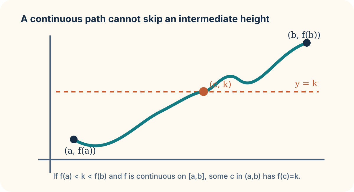
To prove that $x^3-x-1=0$ has a solution between one and two, define $g(x)=x^3-x-1$. This polynomial is continuous on $[1,2]$. Evaluate the endpoints: $g(1)=-1$ and $g(2)=5$. Because zero lies between negative one and five, the IVT guarantees a number $c$ in $(1,2)$ such that $g(c)=0$. Notice that we have proved existence without pretending to have found the root.

The same reasoning supports numerical methods. A sensor calibration function may produce $-0.12\,\mathrm{V}$ at one setting and $0.08\,\mathrm{V}$ at a higher setting. If the model is continuous over those settings, some setting gives $0\,\mathrm{V}$. Bisection then repeatedly tests midpoints to narrow the interval containing a root. IVT supplies the logical guarantee; a numerical algorithm supplies an approximation. Keeping those jobs separate avoids a common overclaim.

How continuity supports derivative work

Continuity does not guarantee differentiability. The function $|x|$ is continuous at zero, but its left slope is $-1$ and its right slope is $1$, so no single tangent slope exists there. A corner is continuous but not differentiable. Differentiability is stronger: every differentiable function is continuous at that point, while some continuous functions have corners, cusps, or other local behavior that prevents a derivative.

This hierarchy helps organize the next unit. Limits ask what nearby values approach. Continuity asks whether the nearby value agrees with the point value. Differentiability asks whether nearby secant slopes settle on one local rate. Each new concept uses the prior one but adds a more demanding agreement condition. Do not replace the tests with a vague visual judgment; use the definition appropriate to the question.

Before leaving this unit, make a three-column table for any suspect point: point value, left/right limits, and conclusion. Then test $h(x)=\frac{x^2-4}{x-2}$ at $x=2$, $j(x)=|x|$ at $x=0$, and $q(x)=\frac1{x-1}$ at $x=1$. State whether each is continuous and give the precise reason. For $j$, add the extra question of whether it is differentiable. This is the bridge from continuity to local slope.

Unit 2 narrative challenge: calibrating a warning threshold

A laboratory monitor reports a corrected signal $S(t)=t^3-4t+1$, where $t$ is a dimensionless calibration setting between $1$ and $2$. The warning threshold is $S=0$. A technician needs a defensible reason to begin a root-search procedure rather than simply trusting a graph. The monitor model is polynomial, but the technician has not yet calculated the exact setting. What facts would prove that at least one calibration setting in the interval triggers the warning threshold?

Do not solve the cubic immediately. First name the theorem that connects endpoint information to an interior solution. Then evaluate the signal at the endpoints, compare each result with the threshold, and check the theorem’s continuity hypothesis. Finally, explain what the conclusion does and does not reveal about the setting. The answer should distinguish a proof of existence from a numerical estimate.

Solution and reasoning

Because $S(t)=t^3-4t+1$ is a polynomial, it is continuous on $[1,2]$. At $t=1$, $S(1)=-2$; at $t=2$, $S(2)=1$. The target $0$ lies between $-2$ and $1$, so the Intermediate Value Theorem guarantees some $c\in(1,2)$ with $S(c)=0$. This proves that a threshold-crossing setting exists. It does not identify the exact value of $c$ or prove that there is only one such value; a numerical method or further analysis would be needed for either claim.

Continuity joins the local language of limits to a global promise about continuous change on an interval. It tells us exactly when a graph’s point value and nearby behavior agree, and the IVT lets us prove that intermediate outputs occur without locating them first. In the derivative unit, we return to secant slopes and ask when their nearby behavior also settles into one value. That limit of slopes will turn continuity’s smooth connection into a measurable local rate.