Antiderivatives and Simple Differential Equations

Differentiation begins with a quantity and produces a rate of change. Antidifferentiation reverses that question: given a rate, what functions could have produced it? An antiderivative of $f$ is any function $F$ whose derivative is $f$. Because constants disappear under differentiation, a rate usually determines a family of possible original quantities rather than one unique function.

This lesson introduces indefinite integrals as notation for those families and shows how an initial condition selects one member. We will also interpret a simple differential equation as a statement about a changing quantity. The next lessons will build definite integrals from sums and then connect accumulated change to antiderivatives through the Fundamental Theorem of Calculus.

By the end, you should find basic antiderivatives, write the constant of integration, verify an answer by differentiating, and use an initial value to solve for the constant. You should attach units to a rate equation and its accumulated quantity. An antiderivative is not merely a reversed exponent maneuver; it is a model for reconstructing change.

Families arise because constants vanish

If $F'(x)=f(x)$, then $(F(x)+C)'=f(x)$ for every constant $C$. The notation

$$\int f(x)\,dx=F(x)+C$$

means “find the family of all antiderivatives of $f$.” The integral sign is read as an indefinite integral here. The differential $dx$ identifies $x$ as the variable of integration. It does not mean a number is being inserted without context.

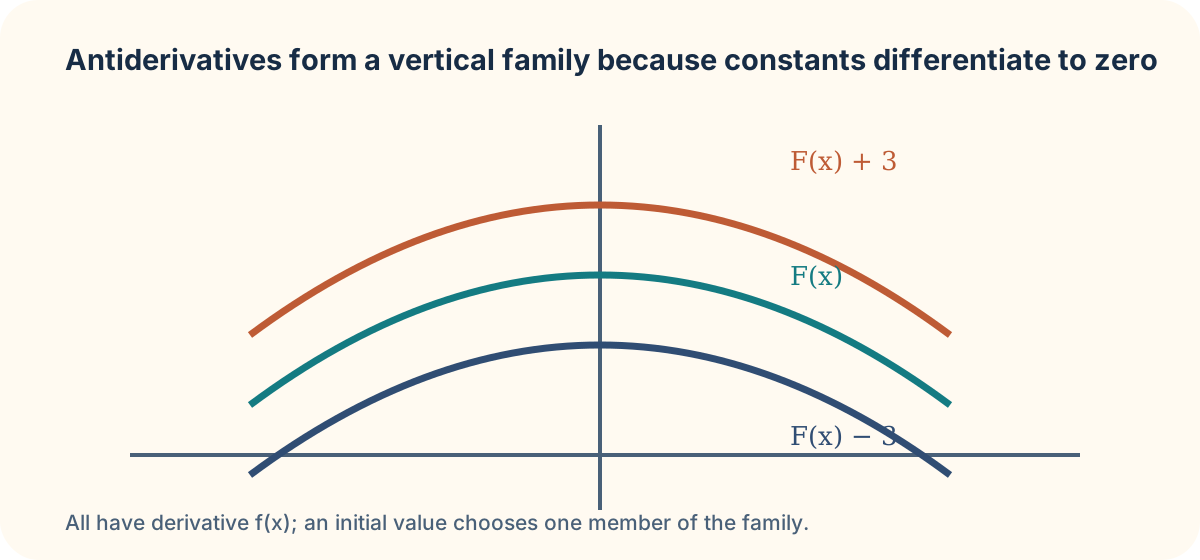
For example, $\int 6x\,dx=3x^2+C$ because the derivative of $3x^2+C$ is $6x$. The constant is essential. Writing only $3x^2$ gives one possible antiderivative, not the complete family. A quick derivative check is the most reliable way to catch a missing coefficient or an incorrect exponent.

Reverse the power rule carefully

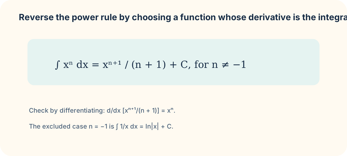
The reverse power rule is

$$\int x^n\,dx=\frac{x^{n+1}}{n+1}+C, \qquad n\ne-1.$$

Increase the exponent first, then divide by the new exponent. For $\int x^4\,dx$, the result is $\frac{x^5}{5}+C$. Differentiating $\frac{x^5}{5}$ returns $x^4$, which verifies the calculation. The rule excludes $n=-1$ because division by zero would result; that special integrand is $\frac1x$, whose antiderivative is $\ln|x|+C$ on intervals that avoid zero.

Linearity still applies. Thus

$$\int(3x^2-4x+5)\,dx =x^3-2x^2+5x+C.$$

Differentiate the result term by term to confirm the original integrand. Do not apply the power rule across an addition inside a nontrivial power, such as $(x+1)^5$, without a suitable substitution; function structure still matters.

Initial values select one physical quantity

A differential equation describes a relationship involving an unknown function and one or more derivatives. If $v'(t)=6t$ in $\frac{\mathrm{m}}{\mathrm{s}^2}$, then velocity has the form $v(t)=3t^2+C$ in $\frac{\mathrm{m}}{\mathrm{s}}$. The rate information alone leaves $C$ undetermined. A condition such as $v(0)=4\,\frac{\mathrm{m}}{\mathrm{s}}$ fixes $C=4\,\frac{\mathrm{m}}{\mathrm{s}}$.

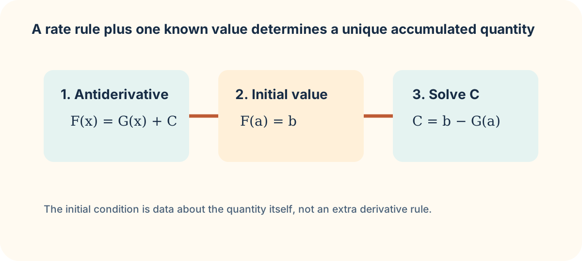
The completed model is $v(t)=3t^2+4$ with velocity units $\frac{\mathrm{m}}{\mathrm{s}}$. If position is needed, integrate velocity once more and use a position initial condition. Each integration introduces a new constant because each recovered layer of accumulation has its own unknown starting level. Units help track the layers: acceleration integrates to velocity, and velocity integrates to position.

Bridge from local rate to total change

An antiderivative gives a function whose local derivative matches a given rate. It does not yet tell us the exact net change over a finite interval without comparing values or using a definite integral. The upcoming Riemann-sum lesson will construct total accumulation by adding many small rate-times-width contributions. The Fundamental Theorem will prove why evaluating an antiderivative at endpoints performs that accumulation efficiently.

Practice by finding an antiderivative of $8t^3-6t$ and checking it by differentiation. Then solve $q'(t)=4t+1$ with $q(0)=7\,\mathrm{L}$, treating $q'$ as a flow rate in $\frac{\mathrm{L}}{\mathrm{min}}$ and $t$ in minutes. State the units of each term and explain what the initial condition contributes. The next lesson makes the accumulation idea visible through areas, sigma notation, and Riemann sums.