Parameters Across Function Families

A function family is a collection of related functions produced by varying parameters. Parameters do more than make graphs look different. They encode initial values, rates, scales, locations, periods, or asymptotic behavior. Their meanings depend on the family and on the units of the modeled quantities. This lesson compares major families so that later calculus results can be interpreted rather than applied to anonymous formulas.

The guiding question is which features change when a parameter changes and which features remain structural. We will compare linear, quadratic, exponential, logarithmic, and trigonometric forms. We will identify parameter meanings through landmarks and units. We will also distinguish a visual fit from a model justified by mechanism or data. The goal is not to memorize a catalog but to build a comparison method.

By the end, you should identify a family from its defining behavior, interpret common parameters, and state relevant invariants. You should explain why the same letter can carry different meanings in different forms. You should use units to evaluate whether a parameter interpretation is coherent. You should also predict which observations would help distinguish competing families. The lesson closes by preparing the average-rate questions that calculus uses to compare change.

Linear and quadratic families

The linear family $f(x)=mx+b$ has constant average rate $m$ on every nonzero interval. The parameter $b=f(0)$ is the vertical intercept when zero belongs to the domain. If $x$ is measured in seconds and $f(x)$ in meters, then $m$ has units of meters per second and $b$ has units of meters. Changing $m$ rotates the line about its intercept, while changing $b$ translates it vertically. Constant rate is the structural invariant.

The quadratic family can be written as $f(x)=a(x-h)^2+k$. Its vertex is $(h,k)$, and its axis of symmetry is $x=h$. The sign of $a$ determines whether the graph opens upward or downward, while $|a|$ controls vertical scale. Average rate is not constant; it changes with the interval location. Symmetry about a vertical line is the central structural feature.

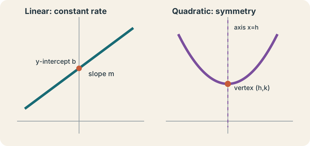
Different algebraic forms reveal different information. Expanded form $ax^2+bx+c$ shows polynomial coefficients and the vertical intercept $c$. Factored form $a(x-r_1)(x-r_2)$ shows zeros when real factors exist. Vertex form shows extrema and symmetry. Rewriting does not change the function, but it changes which parameter relationships are immediately visible. Strategic form choice is part of mathematical reasoning.

Exponential and logarithmic families

An exponential model may be written $P(t)=P_0e^{kt}$. The parameter $P_0=P(0)$ is the initial value, and $k$ is a continuous relative growth rate. Because the exponent $kt$ must be dimensionless, $k$ has units reciprocal to the units of $t$. Positive $k$ produces growth and negative $k$ produces decay. A constant relative rate, rather than a constant additive rate, is the characteristic structure.

A logarithmic function is the inverse of an exponential function after compatible domains and ranges are chosen. In $g(x)=a\ln(x-h)+k$, the input condition is $x>h$, creating a vertical asymptote at $x=h$. The factor $a$ changes vertical scale and orientation, while $k$ translates outputs. Logarithmic growth continues without bound but slows on a linear input scale. Its domain restriction must remain visible in every interpretation.

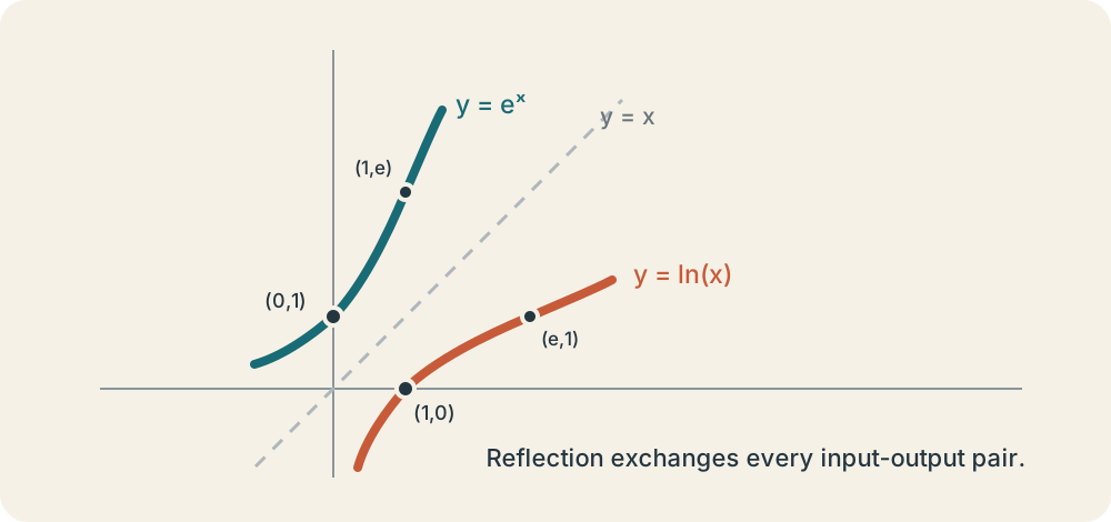
Linear and exponential models can look similar over a short interval. A mechanism helps distinguish them: equal additive change favors a linear family, while equal multiplicative change favors an exponential family. Tables with equal input spacing make that comparison possible. Constant first differences support linear behavior, whereas approximately constant output ratios support exponential behavior. Neither pattern alone proves a real system obeys the model outside the observed range.

Trigonometric families

The sinusoidal family $f(t)=A\sin(B(t-C))+D$ models repeated behavior. The amplitude is $|A|$, the midline is $y=D$, and the period in radians is $\frac{2\pi}{|B|}$. The parameter $C$ shifts the cycle horizontally. A negative $A$ reverses orientation about the midline. Periodicity is the structural invariant.

Units matter inside trigonometric functions. The angle $B(t-C)$ must be dimensionless or interpreted in radians, so $B$ carries reciprocal time units when $t$ is time. The output units belong to both $A$ and $D$ because they determine vertical scale and midline. Adding an output quantity to a dimensionless sine value would be incoherent without the amplitude supplying output units. Dimensional analysis explains the roles of the parameters.

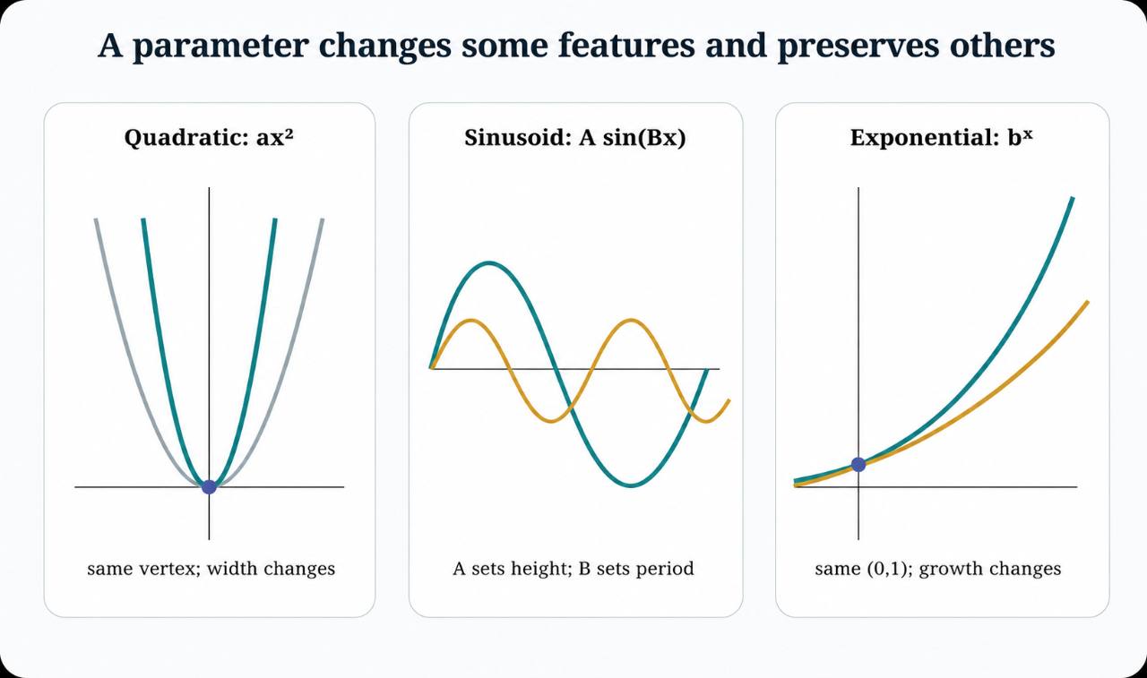
A sinusoidal fit is appropriate only when repeated structure is plausible. A single rise and fall does not prove periodicity. Evidence should include multiple cycles, a physical mechanism, or both. Parameters estimated from a short record can be unstable. A responsible model statement identifies the observed interval and avoids extrapolating cycles without justification.

Compare families by behavior

Begin with domain and range because they can eliminate impossible families. Then inspect intercepts, symmetry, periodicity, asymptotes, and end behavior. Compare equal-step differences and ratios in a table. Finally, interpret parameters in the chosen family and check their units. This routine connects representation evidence with model structure.

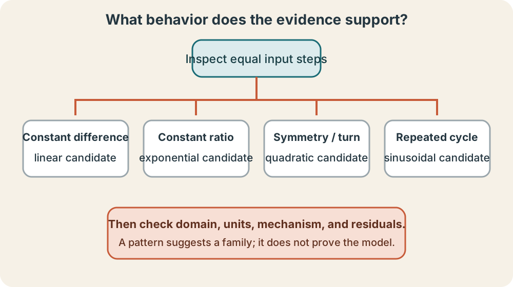
Suppose a quantity increases by about $12$ units during every hour. A linear family is a natural first candidate because additive change is nearly constant. Suppose instead it increases by about $8\%$ during every hour. An exponential family is more natural because multiplicative change is nearly constant. Both conclusions remain provisional until residual patterns and context are examined.

Parameter symbols have no universal meaning apart from their formulas. The letter $a$ can represent quadratic scale, exponential initial value, or sinusoidal amplitude depending on the chosen form. Read a parameter through the operation it performs and the units it must carry. Do not transfer an interpretation merely because the same letter was reused. Mathematical meaning comes from structure, not typography.

Synthesis and transition

Create a comparison table with one row for each major family. Include a representative formula, natural domain restrictions, one invariant feature, and the meaning of two parameters. Add appropriate units to a concrete example in each row. Then explain which evidence would distinguish a linear model from an exponential model and a quadratic model from a sinusoidal segment. The explanation should name both behavior and limitations.

Analyze the model $T(t)=18+6\sin\left(\frac{\pi}{12}(t-4)\right)$, where $T$ is degrees Celsius and $t$ is hours. Identify amplitude, midline, period, and horizontal shift. State the units of every dimensional parameter. Predict maximum and minimum temperatures and the times at which they repeat. Explain why observing fewer than twenty-four hours would weaken a periodicity claim.

Function families organize recognizable kinds of behavior, while parameters select particular members and encode interpretable features. Invariants help identify what remains stable as parameters change. Units and domain restrictions prevent a visually attractive graph from becoming an incoherent model. The next lesson measures how outputs change across intervals. That average-rate framework will reveal the defining constant rate of a line and the interval-dependent rates of nonlinear families.