Radians, Neighborhoods, and Calculus Readiness

Calculus uses several familiar precalculus ideas with unusually precise meanings. Radians connect angle directly to arc length and make trigonometric rates natural. Absolute value expresses distance and therefore describes neighborhoods around a target. Exponent and logarithm laws preserve multiplicative structure but do not distribute across addition. These are not unrelated review topics. They are pieces of the language used to define and compute limits.

This lesson completes the foundations unit by connecting those tools to future calculus work. We will derive the radian relationship, translate absolute-value inequalities into intervals, and audit exponent-logarithm transformations. We will also finish with a cumulative greenhouse-controller narrative. The solution is separated so readers can attempt the problem first. The guiding question is whether the prerequisite ideas can be used with meaning, units, and restrictions intact.

By the end, you should convert between angular and linear quantities using radians, interpret $|x-a|<\delta$ as a neighborhood, and apply exponent and logarithm laws correctly. You should explain why common false distribution rules fail. You should integrate functions, units, rates, domains, and model judgment in the unit challenge. The conclusion then opens Unit 2 by identifying the unresolved need for limits.

Radians connect angle to length

One radian is the central angle that cuts an arc equal in length to the circle’s radius. More generally,

$$\theta=\frac{s}{r},$$

where $s$ is arc length and $r$ is radius measured in the same length unit. The ratio is dimensionless, although the radian label communicates angular meaning. A full circle has arc length $2\pi r$, so it contains $2\pi$ radians.

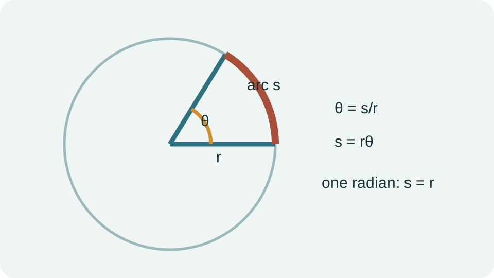
Radians make linear and angular motion connect directly. If a wheel of radius $0.30\,\mathrm{m}$ turns through $4\,\mathrm{rad}$ without slipping, a point on its rim travels $s=r\theta=(0.30\,\mathrm{m})(4)=1.2\,\mathrm{m}$. If angular velocity is $\omega$ radians per second, tangential speed is $v=r\omega$. No degree-conversion factor interrupts the relationship. This simplicity is why calculus formulas for trigonometric derivatives require radian measure.

Degree input changes the scaling. Since $180^\circ=\pi\,\mathrm{rad}$, one degree equals $\frac{\pi}{180}$ radians. A derivative with respect to degrees therefore carries an additional factor. Treating degree and radian inputs as interchangeable changes the rate, even when calculator values look familiar. Always identify the angle unit before interpreting a trigonometric model.

Absolute value describes neighborhoods

The expression $|x-a|$ is the distance between $x$ and $a$ on the real number line. Thus $|x-a|<\delta$ means that $x$ lies within distance $\delta$ of $a$. For positive $\delta$, this is equivalent to

$$a-\delta<x<a+\delta.$$

The parameter $\delta$ controls an input neighborhood centered at the target.

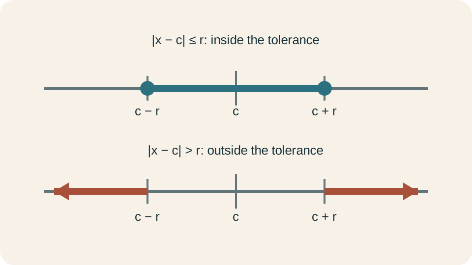
The inequality $0<|x-a|<\delta$ describes a punctured neighborhood. It includes inputs close to $a$ but excludes $x=a$ itself. That distinction will match the idea that limits concern nearby behavior rather than necessarily using the target value. The zero lower bound is not decorative. It explicitly removes the center point.

For an error statement, $|T-20\,{}^\circ\mathrm{C}|<0.5\,{}^\circ\mathrm{C}$ means the temperature lies between $19.5\,{}^\circ\mathrm{C}$ and $20.5\,{}^\circ\mathrm{C}$. Units appear inside the distance comparison because both quantities are temperatures. A tolerance is a radius around a target value. This language later becomes the output side of an epsilon-delta guarantee.

Exponent and logarithm laws preserve structure

For positive bases where the expressions are defined, $a^m a^n=a^{m+n}$ and $\frac{a^m}{a^n}=a^{m-n}$. Powers convert multiplication of like bases into addition of exponents. They do not permit $(a+b)^n=a^n+b^n$. A quick counterexample with $a=b=1$ and $n=2$ disproves that false rule. Structural laws should be tested against simple values when memory is uncertain.

Logarithms reverse exponentiation. For positive $u$ and $v$, $\ln(uv)=\ln u+\ln v$ and $\ln\left(\frac uv\right)=\ln u-\ln v$. Also, $\ln(u^p)=p\ln u$ when the real-domain conditions are satisfied. There is no corresponding rule $\ln(u+v)=\ln u+\ln v$. Logarithms transform products, quotients, and powers—not sums.

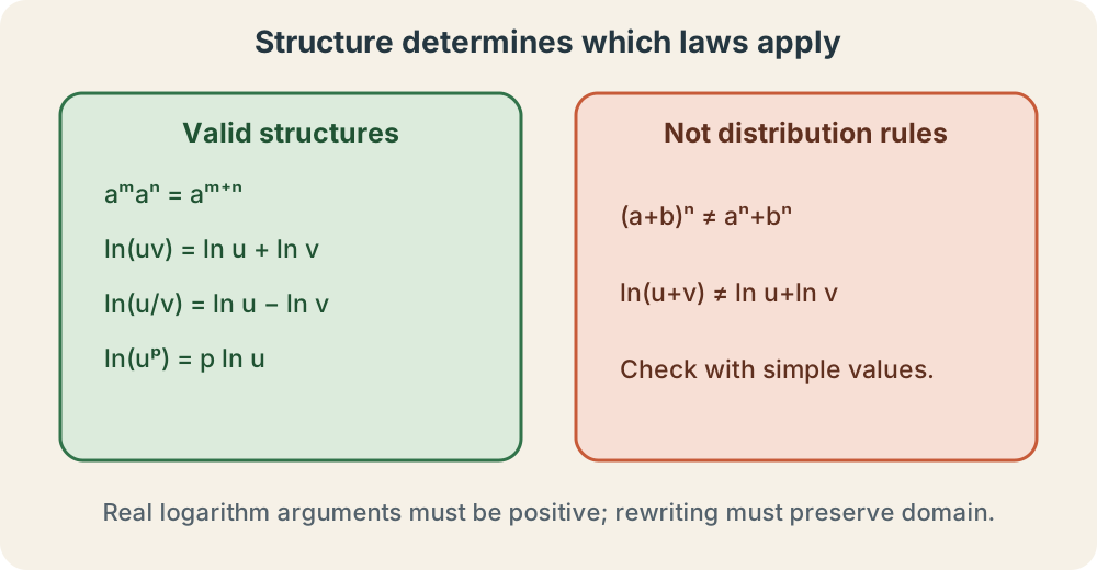
Domain restrictions are inseparable from these laws. A real logarithm requires a positive argument, and a fractional exponent can impose root restrictions. Algebraic rewriting must not silently expand the domain. For example, $\ln(x^2)=2\ln x$ is valid only for $x>0$, whereas the left side also exists for negative nonzero $x$. The domain-aware identity valid for $x\ne0$ is $\ln(x^2)=2\ln|x|$.

A readiness gate

Before beginning limits, verify four capabilities. First, translate functions among words, graphs, tables, and formulas while preserving domains and units. Second, compute and interpret average rates and movable difference quotients. Third, restructure expressions without losing restrictions. Fourth, read radians and absolute-value neighborhoods as geometric quantities. These capabilities support understanding rather than merely faster arithmetic.

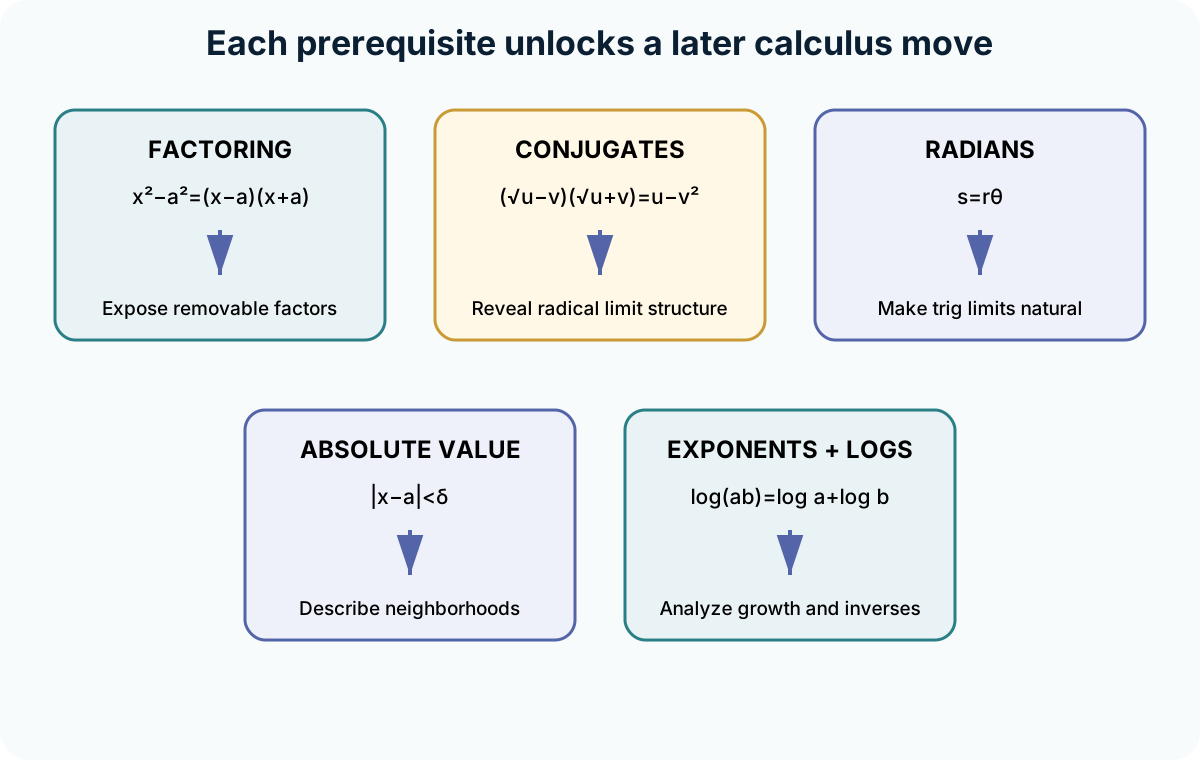
Retrieve the ideas without looking back. Explain why the $h$ in a difference quotient cannot equal zero. Draw $|x-3|<0.4$ on a number line. Convert a $60^\circ$ angle to radians. Give one valid logarithm law and one tempting false law. Factor a difference of squares while naming the excluded denominator input.

If one task fails, repair the specific prerequisite instead of abandoning the course sequence. Difficulty with common denominators calls for targeted algebra practice. Difficulty interpreting $|x-a|$ calls for distance and number-line work. A diagnostic is useful only when it directs the next action. Readiness is a set of revisable skills, not a label attached to a student.

Unit 1 narrative challenge: the greenhouse controller

A greenhouse controller samples air temperature every $2\,\mathrm{min}$. At $t=0\,\mathrm{min}$ the temperature is $18.0\,{}^\circ\mathrm{C}$, at $t=2\,\mathrm{min}$ it is $18.8\,{}^\circ\mathrm{C}$, at $t=4\,\mathrm{min}$ it is $20.1\,{}^\circ\mathrm{C}$, and at $t=6\,\mathrm{min}$ it is $21.0\,{}^\circ\mathrm{C}$. The target is $20.0\,{}^\circ\mathrm{C}$ with an allowed deviation of $0.5\,{}^\circ\mathrm{C}$. The controller must decide when the record first enters the allowed band and how rapidly temperature changes on each sampled interval. The readings alone do not reveal every intermediate temperature.

Before opening the solution, write the allowed band as an absolute-value inequality and as a double inequality. Compute every sampled average rate with units of degrees Celsius per minute. Identify the first recorded time inside the band. Then explain whether the data prove the exact first entry time. Propose one additional measurement that would narrow the uncertainty.

Finally, suppose the controller displays time on a circular twelve-hour dial. Express the $6\,\mathrm{min}$ observation interval as a fraction of one revolution and in radians. Explain why this angular conversion is separate from the temperature-rate calculation. Your response should coordinate representations without mixing their units. End with one sentence naming the new mathematical tool required to infer behavior between increasingly close times.

Open the worked solution after completing your attempt

The allowed band is $|T-20.0\,{}^\circ\mathrm{C}|\le0.5\,{}^\circ\mathrm{C}$, equivalent to $19.5\,{}^\circ\mathrm{C}\le T\le20.5\,{}^\circ\mathrm{C}$. The interval rates are $0.4\,\frac{{}^\circ\mathrm{C}}{\mathrm{min}}$, $0.65\,\frac{{}^\circ\mathrm{C}}{\mathrm{min}}$, and $0.45\,\frac{{}^\circ\mathrm{C}}{\mathrm{min}}$. The first recorded reading inside the band is at $t=4\,\mathrm{min}$. The table does not prove the exact entry time because unsampled behavior between two and four minutes remains unknown.

A measurement at $t=3\,\mathrm{min}$ would divide the uncertain interval, and additional adaptive samples could narrow it further. Six minutes is $\frac{6}{720}=\frac1{120}$ of a twelve-hour revolution because twelve hours contains $720\,\mathrm{min}$. The corresponding angle is $\frac{2\pi}{120}=\frac{\pi}{60}\,\mathrm{rad}$. Angular position and temperature are different outputs, so their units and rates must not be combined. A limit is the next tool needed to describe a stable destination as time intervals shrink.

Closing the foundations unit

Unit 1 has built the objects and tools that calculus acts upon. Functions preserve domains, units, and meanings across representations. Transformations and parameters organize families. Average rates and difference quotients compare change across nonzero intervals. Algebra, radians, and neighborhoods make the later definitions readable.

The greenhouse problem also exposed a boundary of the current tools. A table can identify average changes and recorded entry times, but it cannot automatically determine an instantaneous rate or an exact threshold-crossing time. Making intervals smaller produces better local evidence only if the values stabilize. We need language for that approach without substituting a forbidden zero interval. Unit 2 begins by explaining why calculus needs limits.

End by writing a one-paragraph readiness statement. Name one concept you can explain, one procedure you can justify, and one representation you can translate. Identify any remaining weakness and the exact repair task it suggests. Then state why a limit is conceptually needed before a derivative can be defined. This ending closes the unit while making the next question unavoidable rather than abrupt.