The Instantaneous-Rate Problem

Average rate of change uses two distinct inputs, but ordinary language asks for rates “at” one instant. A speedometer reports a speed now, a sensor reports a heating rate at one time, and a graph has a slope at one point. Substituting the same endpoint twice into an average-rate quotient produces $\frac00$, which is undefined. The physical question remains meaningful even though the direct arithmetic fails. This conflict is one of the problems that created calculus.

This lesson isolates the conceptual problem before introducing formal limit notation. We will compare average velocity with an instantaneous target, connect secant and tangent geometry, and explain why zero cannot be used as an interval width. We will also distinguish a model-defined ideal from a measurement-based estimate. The guiding question is: how can rates across nonzero intervals determine a rate associated with one instant? The next lesson will investigate the behavior of shrinking secants.

By the end, you should explain why $\frac00$ is indeterminate rather than a number, interpret a tangent slope as a local-rate candidate, and describe the role of nearby intervals. You should preserve units through the limiting question. You should also explain why finite measurement resolution does not invalidate an ideal mathematical rate. No formal limit calculation is required yet. The lesson ends by specifying exactly what evidence the next investigation must seek.

Average velocity does not answer every question

Let position be $s(t)=t^2$ meters, with $t$ in seconds. From $t=2\,\mathrm{s}$ to $t=3\,\mathrm{s}$, the average velocity is

$$\frac{s(3\,\mathrm{s})-s(2\,\mathrm{s})}{3\,\mathrm{s}-2\,\mathrm{s}} =\frac{9\,\mathrm{m}-4\,\mathrm{m}}{1\,\mathrm{s}} =5\,\frac{\mathrm{m}}{\mathrm{s}}.$$

This quotient describes net position change per second across the full interval.

The average says nothing certain about velocity at every intermediate time. An object could speed up, slow down, pause, or reverse while producing the same endpoint displacement. The formula $s(t)=t^2$ supplies additional structure, but the endpoint quotient still averages that structure. Asking for velocity exactly at $t=2\,\mathrm{s}$ requires local rather than interval-wide information. The target is associated with one time even though every computable average uses two.

Units remain essential. Position differences carry meters and time differences carry seconds, so every average has units $\frac{\mathrm{m}}{\mathrm{s}}$. If a local velocity is successfully defined, it must carry the same compound unit. Shrinking the interval changes its numerical width but not its physical dimension. A unitless “slope” would omit part of the model.

A zero-width interval is not an interval

The average quotient from $t$ to $t+h$ is

$$\frac{s(t+h)-s(t)}{h},\qquad h\ne0.$$

Setting $h=0$ makes both endpoints identical. The numerator becomes zero because the same position is subtracted from itself, and the denominator becomes zero because no time elapses. Division by zero is undefined. The expression does not acquire meaning merely because the desired answer is called instantaneous.

The form $\frac00$ is called indeterminate because it does not identify one nearby behavior. For $h\ne0$, the quotients $\frac{h}{h}$ and $\frac{2h}{h}$ simplify to $1$ and $2$. Both would display $\frac00$ under illegal direct substitution. Other examples can grow without bound or oscillate. The form reports a need for analysis, not a value.

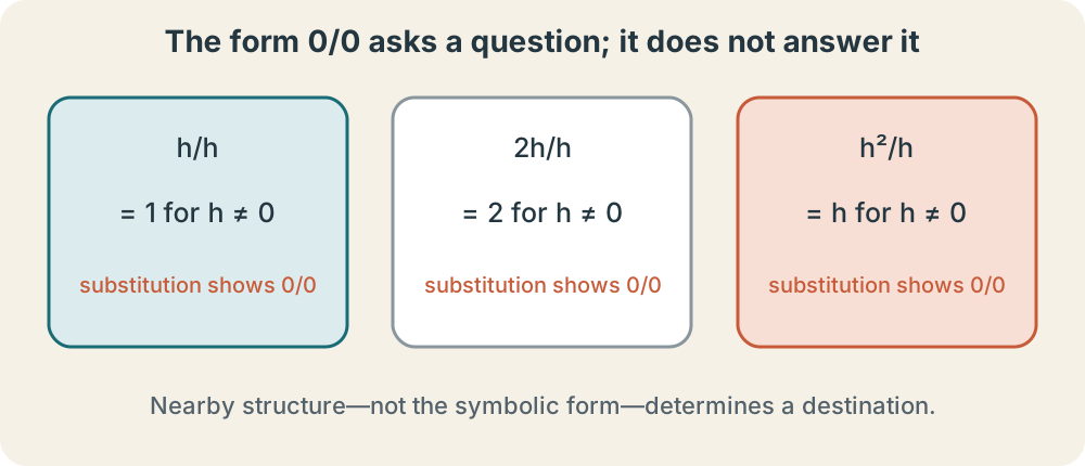
The solution is not to assign a value to division by zero. Instead, retain $h\ne0$ and examine what happens for smaller allowed displacements. This keeps every quotient ordinary and defined. If those quotients stabilize, their destination can define the local rate. The missing zero-width computation is replaced by a controlled statement about all sufficiently small nonzero widths.

Secant lines encode the same problem

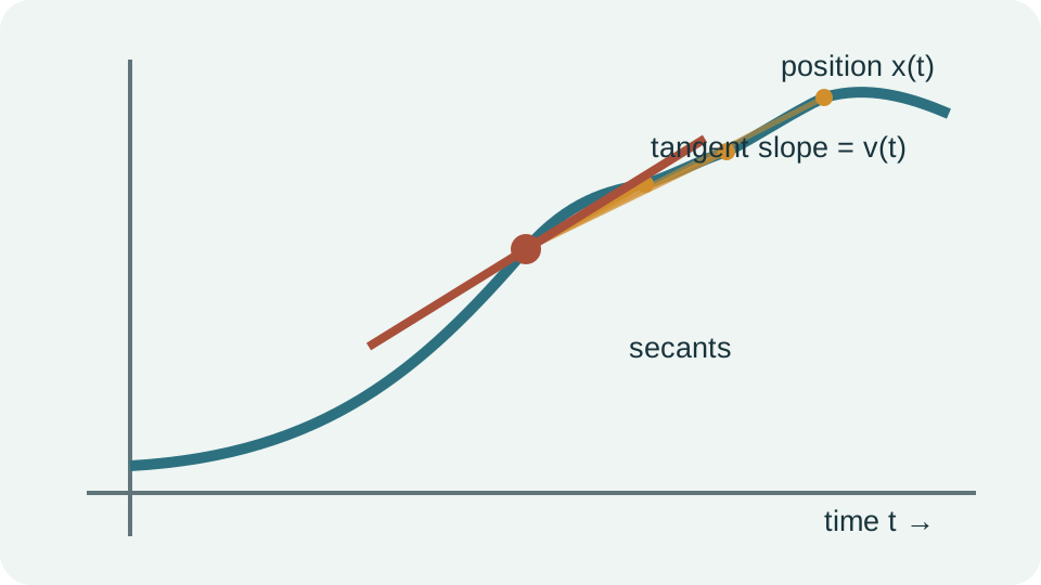
On a position graph, the two interval endpoints determine a secant line. Its slope is the average velocity. Fixing the point at $t=2$ and moving the second point closer produces a family of secants. The lines rotate as their horizontal separation shrinks. A stable limiting line is called the tangent line.

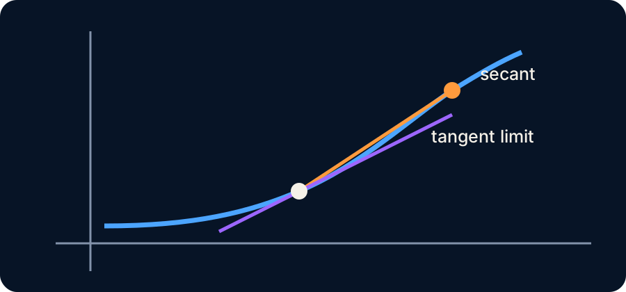
The tangent is not defined as a line that “touches once.” A tangent to a curve can cross the graph, and a line may touch a graph once without representing its local slope. The essential idea is limiting secant behavior. The tangent slope is the destination of nearby secant slopes when that destination exists. This definition coordinates geometry with rate.

For a linear position function, every secant line is already the graph itself and all slopes agree. Nonlinear functions make the problem visible because different intervals produce different slopes. A smooth curve may still look nearly linear when magnified near one point. This local linearity is the structure captured by a derivative later. Limits must first justify the local slope.

Models and measurements answer different versions

A mathematical model such as $s(t)=t^2$ specifies position at every real time in its domain. It permits averages over arbitrarily small nonzero intervals. A physical instrument samples at finite times and with finite resolution. Its estimated rates may become noisy when tiny position differences are divided by tiny time differences. The mathematical ideal and experimental estimate should not be confused.

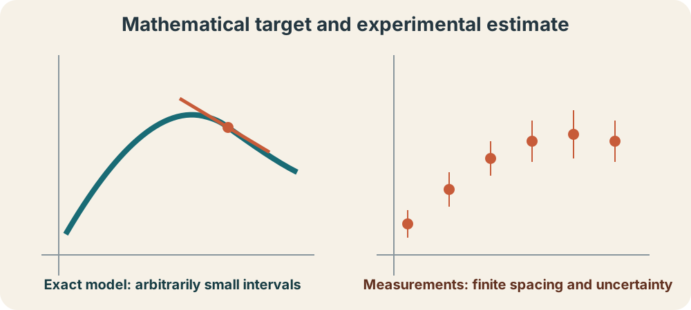
The ideal rate remains useful because it names what an experiment attempts to estimate. If independent smaller-interval estimates stabilize within measurement uncertainty, confidence increases. If they fail to stabilize, the model, instrument, or differentiability assumption may need revision. Calculus does not erase uncertainty. It provides a precise target around which uncertainty can be discussed.

Dimensional analysis supplies a shared check. Every recorded position difference must be compatible with meters, and every interval width with seconds. The quotient therefore carries meters per second at every scale. An instrument may limit precision, but it does not change the quantity’s dimension. Reporting units prevents numerical stabilization from being mistaken for physical interpretation.

Synthesis and transition

For $s(t)=5t^2-3t$ meters, form the average velocity from $t=1\,\mathrm{s}$ to $t=1+h\,\mathrm{s}$. Simplify while retaining $h\ne0$ and attach $\frac{\mathrm{m}}{\mathrm{s}}$ to the quotient. Evaluate it at $h=1\,\mathrm{s}$, $0.5\,\mathrm{s}$, and $0.1\,\mathrm{s}$. Explain why none is automatically the instantaneous velocity. State what kind of shared behavior would justify a local rate.

Then construct two quotients that both yield the form $\frac00$ under substitution but have different nearby constant values. Explain why this disproves the claim that $\frac00=0$. Sketch how their secant slopes would behave. Keep the forbidden target distinct from nearby legal values. Your explanation should use the words interval, destination, and restriction.

The instantaneous-rate problem cannot be solved by collapsing an average-rate interval to zero and dividing. It is solved by studying a family of valid nonzero intervals for a stable destination. Secant slopes express the same question geometrically, while measurement reminds us that evidence has finite resolution. The next lesson performs a systematic two-sided secant investigation. It will determine what stabilization looks like and why approach direction matters.