Newton's Method and Modeling Error

Newton’s Method uses a derivative to improve an estimate of a root, a solution of $f(x)=0$. Starting from a plausible input, draw the tangent line to the graph. Where that tangent meets the horizontal axis is the next estimate. When the graph is well behaved near a simple root and the starting estimate is sensible, the process can converge remarkably quickly.

This lesson also treats numerical results honestly. An iteration can produce a small residual while the mathematical model itself remains only an approximation of the physical situation. Numerical error concerns the calculation’s closeness to a root of the chosen equation. Modeling error concerns whether the chosen equation describes reality adequately. A precise numerical output is not automatically an accurate physical prediction.

By the end, you should derive and use Newton’s update formula, state an appropriate stopping check, identify common failure modes, and distinguish numerical from modeling error. The next unit changes from local rates to accumulated change, beginning with antiderivatives.

Tangent lines produce the iteration

At an estimate $x_n$, the tangent-line approximation is

$$L(x)=f(x_n)+f'(x_n)(x-x_n).$$

Newton’s Method chooses the x-intercept of this line, so set $L(x)=0$ and solve for the next estimate:

$$x_{n+1}=x_n-\frac{f(x_n)}{f'(x_n)}.$$

The denominator requires $f'(x_n)\ne0$. The formula is a tangent-line linearization used to predict where the nonlinear function reaches zero.

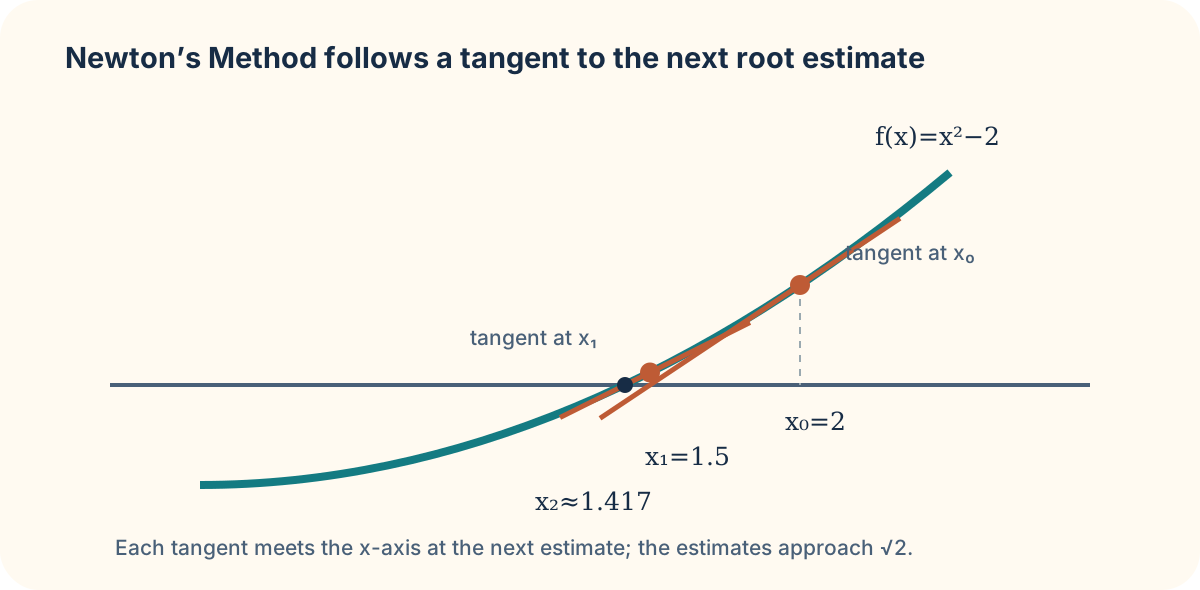
To approximate $\sqrt{2}$, use $f(x)=x^2-2$ and $f'(x)=2x$. Starting with $x_0=1.5$ gives

$$x_1=1.5-\frac{1.5^2-2}{2(1.5)} =1.416\overline{6}.$$

Another iteration produces approximately $1.4142157$, already close to $\sqrt2$. Every value is an approximation; the radical is still the exact root. Record enough digits for the required tolerance, not merely because a calculator displays them.

Run the method with a stopping criterion

An implementation begins with an estimate informed by a graph, a table, or the problem context. At each step compute the new estimate and decide whether the result is sufficiently stable. Common checks include a small step $|x_{n+1}-x_n|$, a small residual $|f(x_{n+1})|$, or both. A small step alone can be misleading near a flat region; a residual directly tests the defining equation.

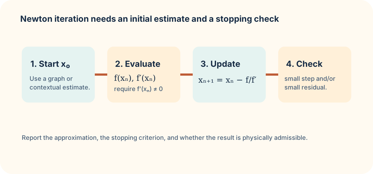
Suppose a calibration model requires a root within $0.001\,\mathrm{V}$ of zero signal. A sensible stopping statement is $|f(x_n)|<0.001\,\mathrm{V}$, together with a domain check on $x_n$. The units of the residual match the function’s output. If the target is an input tolerance instead, specify units for $|x_{n+1}-x_n|$ rather than mixing two different accuracy claims.

Newton’s Method offers no automatic guarantee that a particular initial estimate converges to the intended root. The choice of $x_0$ and the local geometry both matter. A graph or sign-change interval can provide valuable context before iteration begins.

Recognize failure modes and model limitations

If $f'(x_n)$ is zero or very small, the tangent is horizontal or nearly horizontal and its x-intercept can be far away. A poor starting value may jump to a different root, leave the physically meaningful domain, or enter a cycle. Functions with sharp changes, multiple roots, or no root in the intended domain demand extra caution.

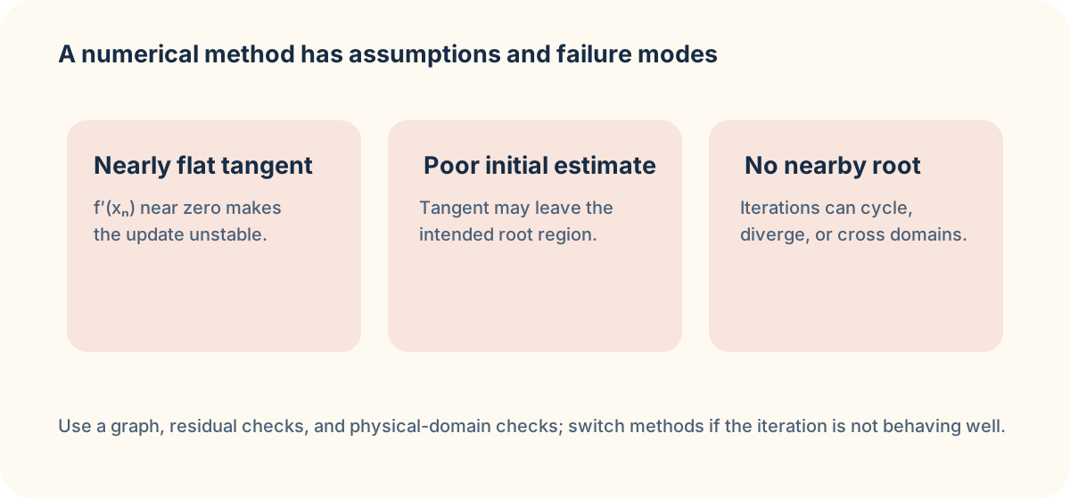
When an iteration behaves poorly, do not keep pressing the update button without diagnosis. Replot the function, choose a new estimate, constrain the domain, or use a bracketing method such as bisection when a guaranteed sign-changing interval is available. The method is a tool with conditions, not a universal root-finding spell.

Numerical error and model error differ in source. If Newton’s iteration stops with a residual of $10^{-8}$, it has found a highly accurate root of the model equation. But if a sensor model neglects friction, temperature drift, or measurement bias, that root may still be a poor estimate of the physical parameter. Report both calculation tolerance and the assumptions that limit the model.

Prepare for accumulation

Newton’s Method uses a derivative to solve an equation locally. The next unit reverses direction: given a rate function, we will seek functions whose derivatives produce that rate. Such functions are antiderivatives. Before moving on, approximate a root of $x^3-x-1=0$ starting from $x_0=1.5$. State the update formula, show at least two iterations, and report a residual. Then explain one reason the resulting numerical root does not by itself validate a real-world cubic model.

Unit 4 narrative challenge: setting a safe release time

A release-control model predicts clearance by $f(t)=t^3-4t-1$, where $t$ is seconds after a mechanism begins moving. The mechanism should release when $f(t)=0$, and a plot suggests the relevant root lies between $2\,\mathrm{s}$ and $3\,\mathrm{s}$. Describe a Newton iteration that could refine the release time. What residual and domain checks would you report before allowing a physical release?

Solution and reasoning

Use $f'(t)=3t^2-4$ and choose a starting estimate in the physically permitted interval, such as $t_0=2.2\,\mathrm{s}$. Iterate $t_{n+1}=t_n-\frac{f(t_n)}{f'(t_n)}$. Stop only when the residual $|f(t_n)|$ is smaller than the specified model-output tolerance and the time remains within the allowed release interval. A small iteration step is useful additional evidence, but it does not replace checking the residual. The calculation estimates a model root; validation of the mechanism still requires that the cubic model’s assumptions be appropriate.