Secants Approaching a Local Rate

The instantaneous-rate problem asks whether valid average rates settle toward one destination as an interval shrinks. A few decimal values are not enough. Evidence should be gathered from positive and negative displacements, connected to a symbolic quotient, and interpreted through secant geometry. This lesson develops that investigation before general limit notation is introduced. The result is a method for recognizing local-rate evidence and diagnosing failure.

We will use $f(x)=x^2$ as a smooth example and $g(x)=|x|$ as a counterexample. Tables, algebra, and graphs will answer different parts of the question. We will distinguish finite-stage values from their proposed destination. We will also explain why approach from both directions matters at an interior point. The guiding question is: when do many changing secant slopes support one local slope?

By the end, you should construct a two-sided secant table, derive its symbolic pattern, and state a local-rate conjecture with appropriate evidence language. You should distinguish positive from negative displacement without confusing either with slope sign. You should identify disagreement at a corner. You should also explain local linearity in words. The next lesson generalizes this approach from secant slopes to arbitrary function values near a target.

Build a two-sided secant table

Fix $f(x)=x^2$ at $x=1$. The secant slope to the point at $1+h$ is

$$\frac{f(1+h)-f(1)}{h}=\frac{(1+h)^2-1}{h}=2+h,qquad h\ne0.$$

The simplified expression represents every legal secant in the family. It also predicts how the slope depends on displacement.

Use $h=1$, $0.5$, $0.1$, $0.01$, and corresponding negative values. The slopes are $3$, $2.5$, $2.1$, $2.01$ from the right and $1$, $1.5$, $1.9$, $1.99$ from the left. The finite values do not become identical. They move closer to the shared number $2$. Stabilization concerns a destination, not eventual equality at a nonzero displacement.

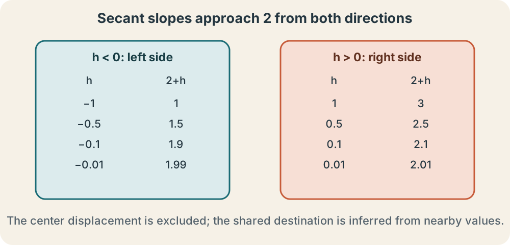
Organize the table into left and right columns rather than one unsorted list. This makes directional evidence visible. Include the moving input $1+h$ so the geometry remains connected to the arithmetic. Do not include $h=0$ as a row because the original quotient is undefined there. The missing center is the question, not a data point.

Read the graph and algebra together

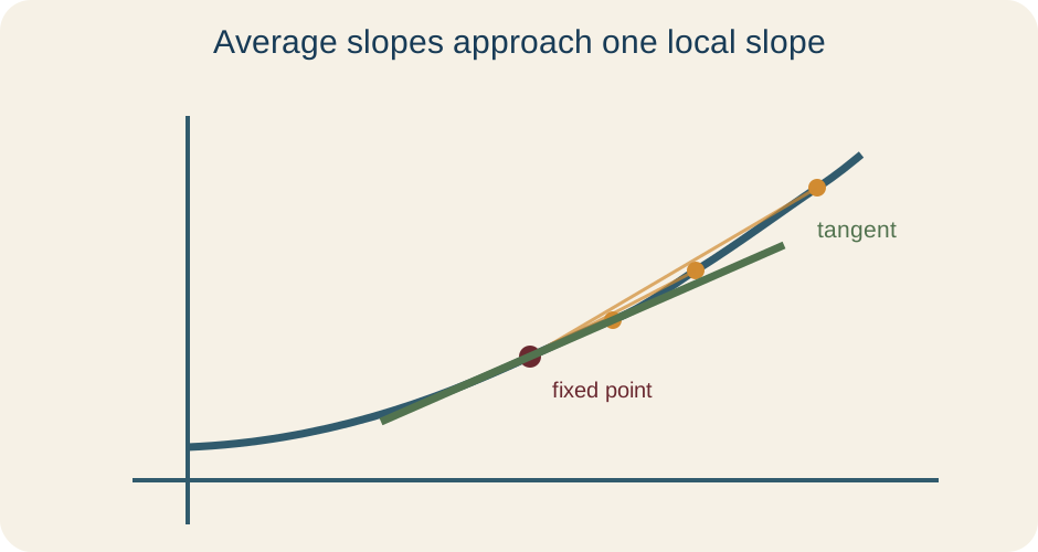
Each table row corresponds to a secant line through $(1,1)$ and $(1+h,(1+h)^2)$. Positive $h$ places the moving point to the right, while negative $h$ places it to the left. As $|h|$ decreases, both families of lines rotate toward the line of slope $2$. The graph supplies spatial meaning to the numerical stabilization. The algebra explains why the value $2$ is not a coincidence of selected samples.

The expression $2+h$ can be made as close to $2$ as desired by making $|h|$ sufficiently small. Their distance is $|(2+h)-2|=|h|$. Thus an input-displacement tolerance immediately controls the slope error. This statement goes beyond a finite table. It anticipates the epsilon-delta idea without requiring its full notation yet.

The tangent line candidate at $(1,1)$ is $y-1=2(x-1)$. Near $x=1$, the parabola and line are visually close because their vertical difference is $(x-1)^2$. That error is second order in the horizontal displacement. Local linearity means a smooth function increasingly resembles an appropriate line under magnification. The derivative will name the line’s slope.

Direction is part of the evidence

At an interior input, allowed nearby values normally occur on both sides. Positive displacement samples the right and negative displacement samples the left. A proposed local rate must be compatible with both directional families. Examining only positive $h$ can miss a corner, cusp, jump, or other disagreement. Two-sided evidence is a requirement, not redundant checking.

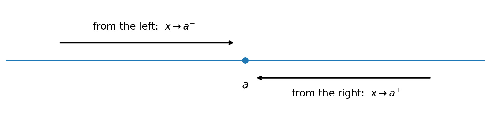
The sign of $h$ does not determine the sign of the secant slope. For $x^2$ at $x=1$, negative $h$ values near zero still produce positive slopes. The displacement sign locates the moving input relative to the base. The slope sign describes whether output rises or falls across the ordered interval. Confusing these roles produces false directional conclusions.

At a domain endpoint, only one side may be available. For $f(x)=\sqrt{x}$ at zero, negative real inputs are excluded, so right-side secants provide the relevant endpoint evidence. It would be wrong to invent left-side inputs. Domain analysis determines which directions must be checked. The next two lessons formalize this distinction with one-sided limit notation.

A corner shows why agreement matters

For $g(x)=|x|$ at $x=0$, the secant quotient is

$$\frac{|h|-0}{h}=\frac{|h|}{h}.$$

For every positive $h$, the value is $1$. For every negative $h$, it is $-1$. Each directional family is stable, but the two destinations disagree.

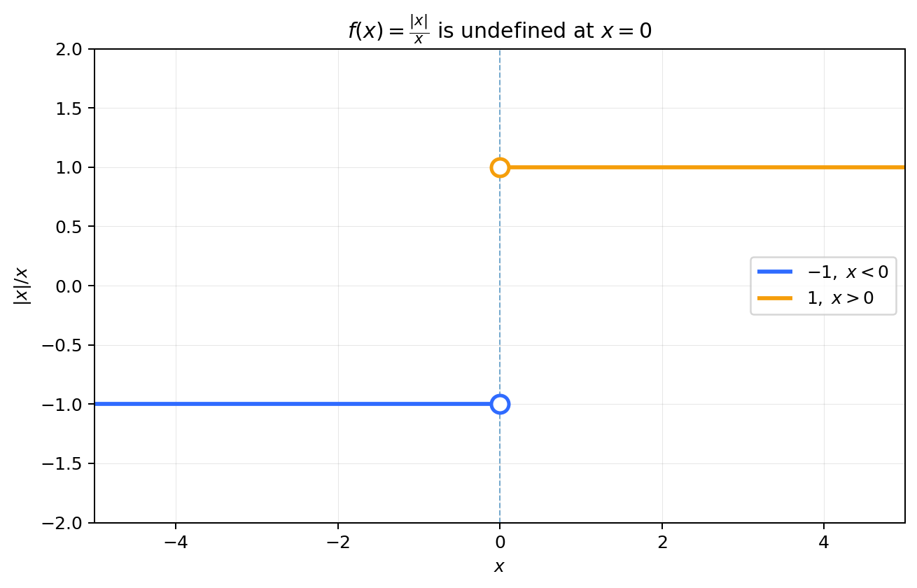
The graph has a corner at the origin. A right-side tangent candidate would have slope $1$, while a left-side candidate would have slope $-1$. No single line describes the graph’s first-order behavior from both sides. The failure is not caused by noisy values or insufficient sampling. It is a genuine structural disagreement.

This example disproves the claim that every shrinking interval produces an instantaneous rate. Calculus defines local rates only where the limiting secant behavior supports one value. A function can be perfectly defined and continuous at a point while lacking a derivative there. Existence must be established rather than assumed. Counterexamples make the definition necessary.

Evidence, conjecture, and proof

A table suggests behavior through finitely many sampled displacements. A graph suggests spatial structure at a chosen resolution. Algebra can establish an exact formula for every allowed displacement. A complete investigation coordinates these representations. It also labels a conclusion as an estimate, conjecture, or proof according to the strength of support.

For the quadratic example, the identity $2+h$ and the distance calculation $|(2+h)-2|=|h|$ provide exact control. For experimental motion data, no exact symbolic identity may be available. Smaller-interval estimates can still support a practical approximation with stated uncertainty. Mathematical proof and empirical estimation answer related but different questions. Neither should impersonate the other.

An investigation should stop when the relevant claim is justified, not when a table has many rows. Repeating more decimal samples cannot by itself turn numerical evidence into proof. Instead, look for a structural relation or theorem that controls all sufficiently small allowed displacements. This shift from examples to guarantees is central to calculus. Formal limit language will make it explicit.

Synthesis and transition

Repeat the investigation for $f(x)=x^2$ at $x=3$. Derive the quotient, create a two-sided table, and predict the local slope. Write the tangent-line candidate through $(3,9)$. Explain how the symbolic form controls the slope error. Then state which parts of your conclusion come from algebra, graph, and table.

Next investigate $g(x)=|x-2|$ at $x=2$. Compute positive and negative displacement quotients and sketch representative secants. State why each directional destination exists but no shared local slope does. Compare this failure with the quadratic success using the words direction, destination, and agreement. Do not write only “undefined.”

Shrinking secants support a local rate when their slopes approach one destination from every required direction. Tables display stabilization, graphs display rotating lines and local shape, and algebra can control the full family. A corner reveals why directional agreement cannot be assumed. The next lesson removes the secant-specific setting and asks what it means for arbitrary function outputs to approach a value. That generalization is the concept of a limit.