Computing Nontrivial Limits

Direct substitution is useful partly because it identifies the cases that need more work. A finite real value may certify a continuous calculation; the form $\frac00$ does neither. It says the numerator and denominator both vanish at the target, leaving nearby structure unresolved. Computing a nontrivial limit means transforming the expression into one that agrees nearby and can be evaluated with a valid limit law. The target point itself may remain excluded throughout.

This lesson turns method selection into a disciplined process. Factoring handles polynomial differences, conjugates handle radical differences, and common denominators handle nested rational differences. Each method aims to reveal a common factor or an equivalent nearby form. We will preserve restrictions while simplifying. The guiding question is: what algebraic structure is hiding behind the indeterminate form? The next lesson explains how to make “nearby” mathematically precise.

By the end, you should diagnose the expression type, select a method, and write restrictions beside each equivalent line. You should explain why cancellation establishes local equivalence rather than repairing the original point. You should reject illegal term cancellation. You should also distinguish a removable hole from a vertical asymptote. The central skill is structural reasoning, not performing a memorized sequence of moves.

Begin with the diagnostic, not the answer

For

$$\lim_{x\to2}\frac{x^2-4}{x-2},$$

substitution produces $\frac00$. This is indeterminate: the form alone does not determine the destination. The denominator signals that $x=2$ is excluded from the original quotient. We must therefore investigate allowed inputs near two. Writing the restriction before algebra prevents a later simplified expression from being misread as the original function.

An ordinary zero denominator with a nonzero numerator suggests unbounded behavior rather than a removable factor. For example, $\frac{x+1}{x-2}$ has numerator three and denominator zero at two. Factoring will not create a common $(x-2)$ factor. The nearby graph has a vertical asymptote. Diagnose before selecting a tool.

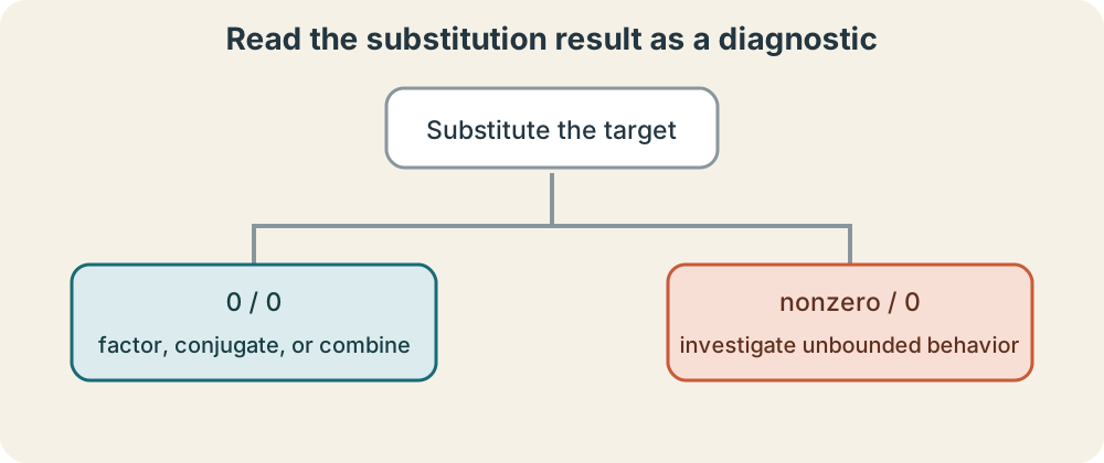
The form $\frac00$ is a request to inspect structure, not a guarantee that the limit exists. A piecewise jump and an oscillating quotient can also defeat a finite limit. Earlier directional analysis still applies. Algebra works when it establishes valid equality on a punctured neighborhood. It cannot manufacture agreement that nearby behavior lacks.

Factor polynomial differences

The numerator $x^2-4$ factors as $(x-2)(x+2)$. Thus

$$\frac{x^2-4}{x-2}=x+2, \qquad x\ne2.$$

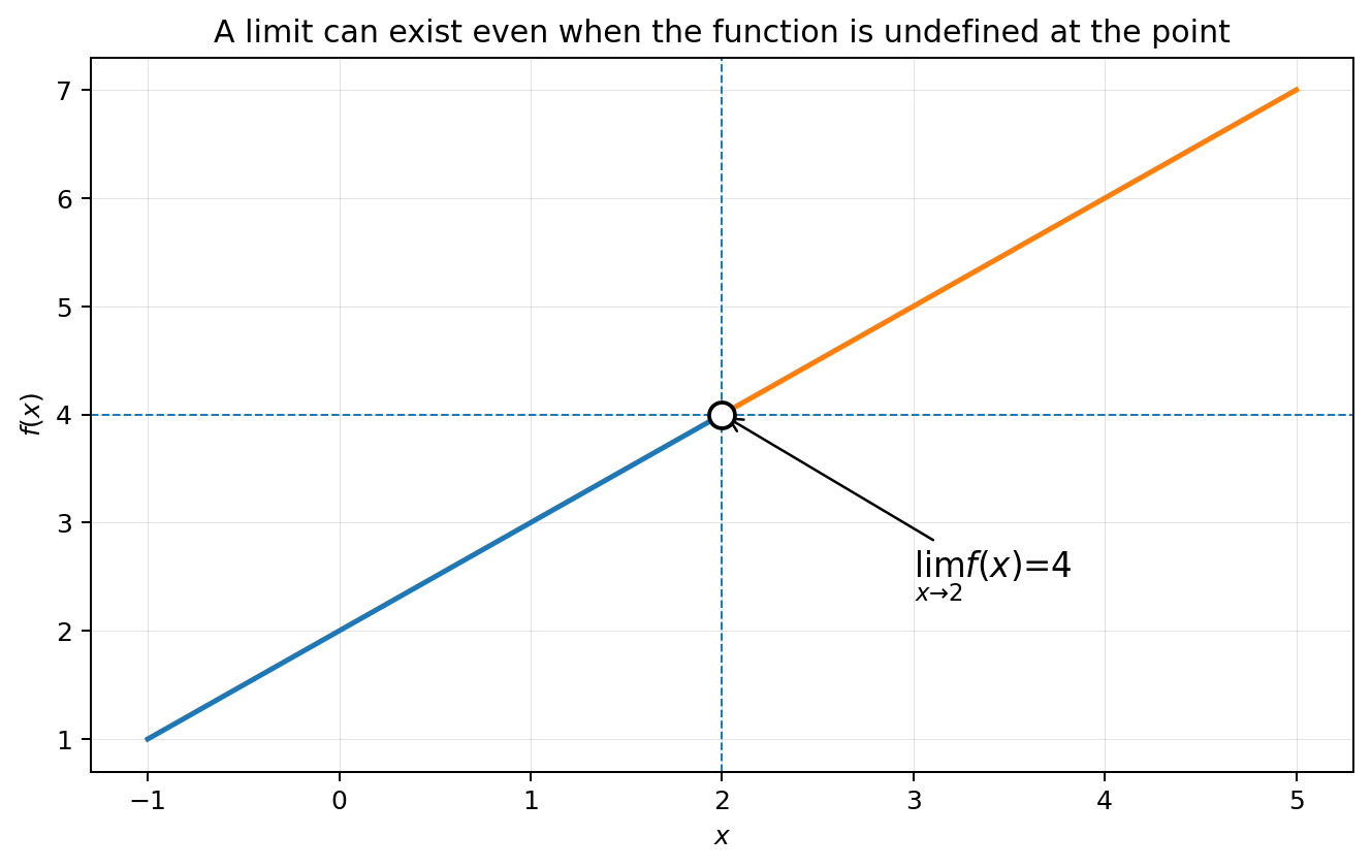
The expressions agree for every allowed input near two. Limit laws now give $\lim_{x\to2}(x+2)=4$. The limit is four even though the original quotient remains undefined at two.

Choose factorization patterns that match the obstructing denominator. Differences of squares use $u^2-v^2=(u-v)(u+v)$. Differences of cubes use $u^3-v^3=(u-v)(u^2+uv+v^2)$. Factoring by grouping can reveal a shared factor in higher-degree expressions. Expanding first often hides the exact feature needed for cancellation.

Cancellation applies to factors, never to individual terms in a sum. The expression $\frac{x+2}{x+2}$ can simplify, but $\frac{x+2}{x}$ cannot become two by “cancelling x.” Parentheses and factored form make the legal operation visible. Every cancellation assumes the factor is nonzero on the nearby domain. State that assumption.

Rationalize radical differences

For

$$\lim_{x\to4}\frac{\sqrt{x}-2}{x-4},$$

factoring the denominator alone does not expose a matching radical factor. Multiply numerator and denominator by the conjugate $\sqrt{x}+2$. The numerator becomes $x-4$ through a difference of squares. That factor cancels for $x\ne4$, leaving $\frac1{\sqrt{x}+2}$.

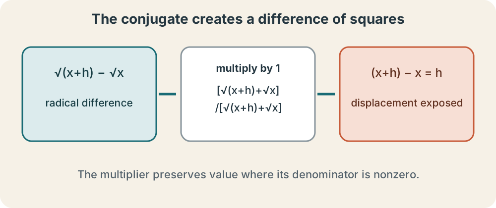
The remaining expression is continuous at four, so substitution gives $\frac14$. The original domain condition $x\ge0$ and the exclusion $x\ne4$ belong to the transformation, even if the final expression is defined at four. The limit calculation uses nearby equality; it does not claim that the original quotient has acquired a value.

Conjugates are not a ritual for every square root. They are useful when a difference of radicals blocks comparison and the product will create a difference of squares. A sum of radicals may call for another method. Ask what the multiplier changes. A valid conjugate ratio equals one wherever its denominator is nonzero, preserving the nearby value.

Combine nested rational expressions

For

$$\lim_{x\to0}\frac{\frac1{x+1}-1}{x},$$

combine the numerator first:

$$\frac1{x+1}-1=\frac{1-(x+1)}{x+1}=\frac{-x}{x+1}.$$

Dividing by $x$ gives $-\frac1{x+1}$ for $x\ne0$ and $x\ne-1$. The limit is then $-1$.

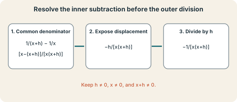
The subtraction sign must distribute across the full second numerator. Writing $1-x+1$ instead of $1-(x+1)$ changes the algebra. Treat the outer quotient as a separate layer until the inner difference has been simplified. Then list every denominator restriction from the original expression. Simplification may hide one restriction but cannot erase it.

Common denominators are also useful when two rational functions must be compared near a target. The goal is to reveal the difference in a form that contains the vanishing displacement. Do not cancel across addition before combining into a single fraction. Factor after the numerator is organized. Structure determines order.

Verify the nearby claim

After simplification, ask three questions. First, is the transformed expression equal to the original for all nearby allowed inputs? Second, is the transformed expression continuous at the target? Third, have every original exclusion and new domain condition been recorded? If the answers are yes, direct substitution into the transformed expression computes the limit. The logic is local and complete.

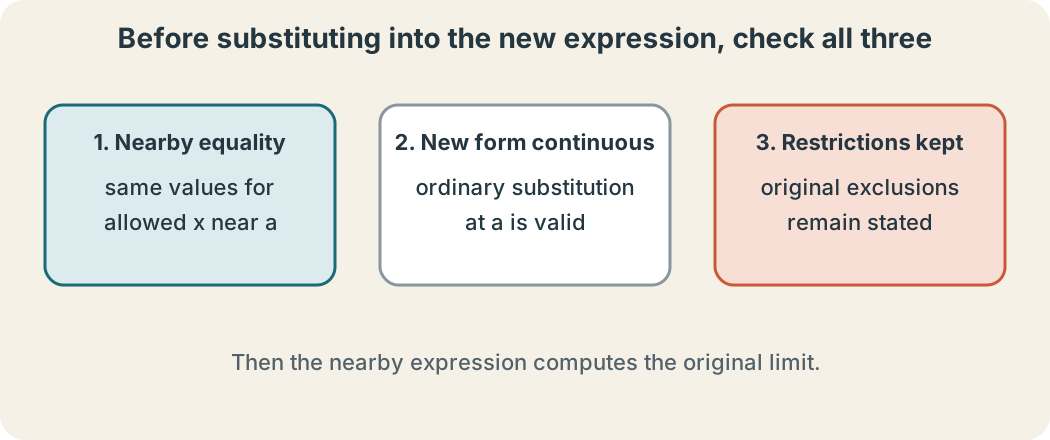
Compare two targets for $\frac{x^2-4}{x-2}$. At two, factoring produces a removable hole and a finite limit of four. At no other denominator zero is present because two is the only excluded point. By contrast, for $\frac{x+1}{x-2}$ at two, no cancellation occurs and the quotient is unbounded. Similar fraction typography does not imply similar local behavior.

Numerical tables and graphs can check a result, but they should not replace the nearby equality argument. A table near four for the radical example should show values near one fourth. A graph should show an open point at the target. These representations communicate the result. The algebra establishes why it holds throughout a punctured neighborhood.

Synthesis and transition

Compute the limits of $\frac{x^2-9}{x-3}$ as $x$ approaches three, $\frac{\sqrt{x+5}-3}{x-4}$ as $x$ approaches four, and $\frac{\frac1{x+2}-\frac12}{x}$ as $x$ approaches zero. For each, state the diagnostic form, name the selected method, preserve restrictions, and then substitute into the continuous nearby expression. Explain why no original point value is needed.

Then construct one rational expression with a removable hole and one with a vertical asymptote at the same target. Use factoring to justify the first classification and a nonzero numerator-over-zero denominator check to justify the second. Sketch both graphs with open points or asymptotic branches. Explain why one has a finite limit and the other does not.

Nontrivial finite limits are computed by revealing valid nearby structure. Factoring, conjugates, and common denominators are chosen because they expose the cancellation or equality the original form hides. Restrictions remain part of the argument, and $\frac00$ remains a diagnostic rather than an answer. The next lesson makes the phrase “sufficiently close” exact through epsilon and delta. It turns observed local control into a formal definition.