Linearization and Differentials

A derivative gives a tangent slope at one input. Linearization turns that slope into a practical local model. Near a chosen base point, a differentiable curve is well approximated by its tangent line. This is calculus’ first systematic approximation tool: replace a complicated function by a simple line only in a clearly stated neighborhood where the replacement is justified.

This lesson connects tangent geometry, small changes, and measurement units. The phrase “approximately equal” will be treated honestly. It is not an invitation to use a line everywhere. A tangent line agrees best near its point of contact, and the approximation error normally grows as the input moves away. Differentials give a compact way to estimate the corresponding small output change.

By the end, you should construct a linearization, use it to estimate a nearby value, interpret $dy=f'(a)dx$ with units, and identify the source of approximation error. You should also distinguish an exact tangent-line equation from an approximate prediction made with that line. The next lesson uses higher derivatives to ask how rates themselves change.

Build the tangent-line model

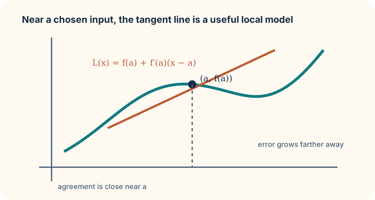
For a differentiable function $f$ at a base input $a$, the linearization is

$$L(x)=f(a)+f'(a)(x-a).$$

The constant term $f(a)$ makes the line pass through the point $(a,f(a))$. The factor $f'(a)$ supplies its slope. The final factor $(x-a)$ measures displacement from the base input, not displacement from zero. Each piece is necessary: remove any one and the expression no longer describes the tangent line at the selected point.

To estimate $\sqrt{4.1}$, use $f(x)=\sqrt{x}$ with base point $a=4$. We know $f(4)=2$ and $f'(x)=\frac{1}{2\sqrt{x}}$, so $f'(4)=\frac14$. The linearization is $L(x)=2+\frac14(x-4)$. Therefore

$$\sqrt{4.1}\approx L(4.1) =2+\frac14(0.1) =2.025.$$

The approximation is credible because $4.1$ lies close to the convenient base input four. The calculation does not claim that the square root function equals its tangent line. It says the tangent line gives a controlled first estimate near that input.

Differentials describe small predicted changes

Let $dx$ denote a small input change from the base input. The corresponding linearized output change is

$$dy=f'(a)dx.$$

Here $dy$ is a differential, or predicted change from the tangent-line model. The actual change is $\Delta y=f(a+dx)-f(a)$. For small $dx$, $dy$ approximates $\Delta y$. The two symbols are related but not identical; writing them distinctly prevents an approximation from becoming an accidental equality.

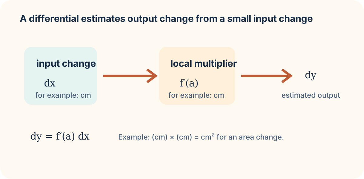
For the area of a circle, $A(r)=\pi r^2$, so $dA=2\pi r\,dr$. At radius $r=10\,\mathrm{cm}$ and a small radius measurement change $dr=0.02\,\mathrm{cm}$,

$$dA=2\pi(10\,\mathrm{cm})(0.02\,\mathrm{cm}) =0.4\pi\,\mathrm{cm}^2.$$

The units resolve naturally: a rate of area with respect to radius has units of centimeters, and multiplying by a radius change in centimeters gives square centimeters. This makes differentials valuable in measurement contexts, where the question is often how a small input uncertainty affects an output uncertainty.

State where the approximation is trustworthy

The derivative captures first-order change. It does not encode all curvature. If the graph bends noticeably, a tangent line can miss the actual function more strongly as the input moves away from the base point. A responsible approximation names its base point, its input change, and its approximate character. A numerical answer without those conditions can look more certain than the mathematics supports.

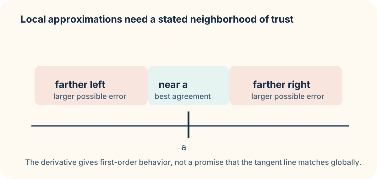
For $f(x)=x^2$ at $a=2$, the linearization is $L(x)=4+4(x-2)$. At $x=2.1$, it predicts $4.4$, while the exact value is $4.41$. The error is $0.01$. At $x=3$, the same line predicts $8$, but the exact value is $9$; the error is much larger. The tangent line remains exact at the base point and has the correct slope there, but it is not a global substitute for the parabola.

Higher derivatives help explain this trend. A nonzero second derivative indicates that the slope changes, so a fixed tangent line will gradually fail to follow the curve. We will use second derivatives soon to study concavity and motion. For now, use the derivative as a local sensitivity: it tells how much the output responds per small unit input change at the chosen operating point.

Practice with a local model

Construct the linearization of $f(x)=x^3$ at $a=2$, then use it to estimate $2.02^3$. Identify $f(a)$, $f'(a)$, and $x-a$ before multiplying. Next, if a cube’s side length is measured as $5.00\,\mathrm{cm}$ with a possible small error of $0.01\,\mathrm{cm}$, use $V(s)=s^3$ and a differential to estimate the induced volume change in $\mathrm{cm}^3$.

In each case, say why the derivative method is sensible: the new input is close to the base input, and the tangent line records the correct first-order response there. Then say what would make it less sensible: a large input change, a non-differentiable base point, or a required error tolerance tighter than the approximation can support. This discipline will carry into optimization, numerical methods, and all later applied calculus work.