Numerical Integration and Average Value

Not every accumulated quantity arrives with an antiderivative that is easy to write, and experimental data may provide only sampled values. Numerical integration estimates a definite integral from finite information. It does not replace the definition of an integral; it applies the same rate-times-width idea with a chosen local approximation on each subinterval.

This lesson compares midpoint and trapezoidal approximations, explains what their units and errors mean, and introduces average value as a constant height that produces the same accumulated area as a varying function. The important habit is to label estimates honestly. A numerical rule produces an approximation unless a special situation makes it exact.

By the end, you should construct midpoint and trapezoidal estimates, report their units, recognize how refinement affects them, and compute and interpret average function value. The next unit applies integration to regions, volumes, work, and course synthesis.

Approximate with a local shape

The midpoint rule treats the function as constant at a representative midpoint in each subinterval:

$$M_n=\sum_{i=1}^{n}f(m_i)\Delta x.$$

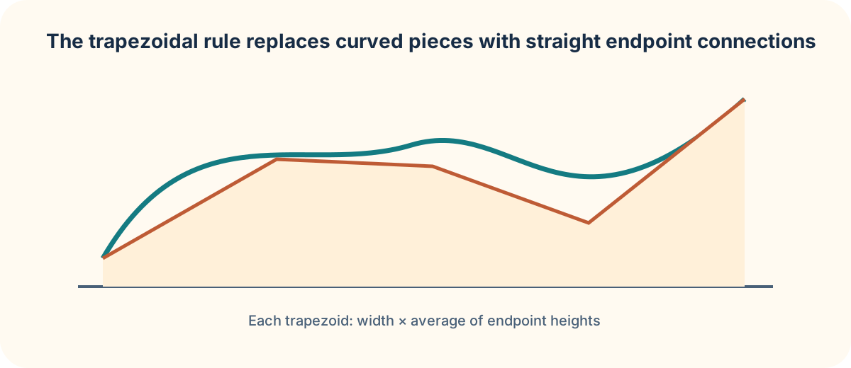
The trapezoidal rule connects endpoint values by a straight segment, then adds trapezoid areas:

$$T_n=\sum_{i=1}^{n}\frac{f(x_{i-1})+f(x_i)}{2}\Delta x.$$

Both formulas approximate $\int_a^bf(x)\,dx$. Their meaning remains height times width summed across the partition.

For a rate measured in $\frac{\mathrm{L}}{\mathrm{min}}$, each numerical contribution has liters after multiplication by a time width in minutes. Thus the final approximation estimates accumulated volume, not a rate. Preserve the units even when a table lists only numbers; the calculation’s dimensional meaning is a built-in error check.

Compare rules and error thoughtfully

Midpoint and trapezoidal rules use different information. The midpoint rule samples one interior height per interval. The trapezoidal rule uses endpoint heights and a linear connection. Neither rule is automatically an overestimate or underestimate without information about concavity. For a concave-up function, trapezoids tend to lie above the curve while midpoint rectangles tend to lie below; concave-down behavior reverses this tendency.

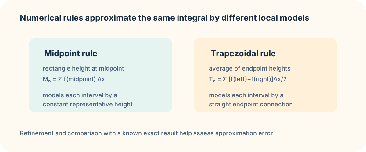
Refining the partition usually improves a reliable approximation for a smooth function, but data noise can complicate this in experiments. If an exact integral is available, compare the approximation to the exact result. If not, compare successive refinements or use an error bound justified by information about derivatives. Never claim an exact value merely because a displayed decimal has many digits.

For a table of flow rates, use the stated sampling scheme. Treating irregularly spaced time readings as equal-width data changes the model. Each trapezoid must use its own interval width. A carefully written numerical setup is often more valuable than an unlabelled final decimal.

Average value is an equal-area height

The average value of an integrable function on $[a,b]$ is

$$f_{\mathrm{avg}}=\frac{1}{b-a}\int_a^bf(x)\,dx.$$

The numerator is total signed accumulation. Dividing by interval width produces an average height in the same units as $f$. Geometrically, it is the height of a rectangle over $[a,b]$ with the same signed area as the region under the function.

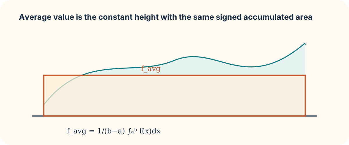
If $v(t)$ is velocity in $\frac{\mathrm{m}}{\mathrm{s}}$, its average value over time is average velocity, with units $\frac{\mathrm{m}}{\mathrm{s}}$. It is displacement divided by elapsed time, not total distance divided by time unless velocity remains nonnegative. Context determines which average is meaningful.

The Mean Value Theorem for Integrals adds an existence claim: under appropriate continuity conditions, some input $c$ has $f(c)=f_{\mathrm{avg}}$. It does not say every input has that value or identify a unique $c$. This is another instance of calculus linking a global average to a local value.

Practice and transition

Use the trapezoidal rule with two equal subintervals to estimate $\int_0^4x^2\,dx$, then compare it to the exact value. State whether the function is concave up and predict the direction of the trapezoidal error. Next find the average value of $f(x)=x^2$ on $[0,3]$ and interpret it as an equal-area rectangle height.

These methods return us to the concrete meaning of integration: accumulated signed contribution. In the next lesson, we subtract one accumulated region from another to find area between curves. Keep track of which function is above on each interval; integration remains sensitive to sign and order.