The Derivative as a Function

The expression $f'(a)$ answers a local question at one input: what is the tangent slope or instantaneous rate when $x=a$? Replacing the fixed input $a$ with the variable $x$ creates a new function. The derivative function $f'$ takes an input location and returns the local rate at that location. This shift is important because calculus rarely asks only for one isolated rate. We want to know where a quantity increases, decreases, levels off, or changes most rapidly across an entire domain.

This lesson treats $f'$ as a full mathematical object. We will interpret its input and output, connect its signs to the shape of $f$, estimate it from a table, and distinguish its domain from the original function’s domain. Shortcut differentiation rules will arrive next. Their purpose is to calculate this rate function efficiently, not to replace the local-rate meaning established here.

By the end, you should be able to say in words what $f'(x)$ and $f'(a)$ mean, infer rising and falling behavior from derivative signs, and estimate a derivative value from nearby data. You should also avoid reading a derivative graph as though it were a graph of the original quantity. The y-values of $f'$ are slopes or rates, not usually the original outputs.

A function that returns slopes

The definition of the derivative function is

$$f'(x)=\lim_{h\to0}\frac{f(x+h)-f(x)}{h},$$

provided the limit exists. The input $x$ is a location in the domain of the original function. The output $f'(x)$ is the limiting slope at that location. A derivative may have a smaller domain than the original function because a function can exist at a corner or discontinuity where no unique tangent slope exists.

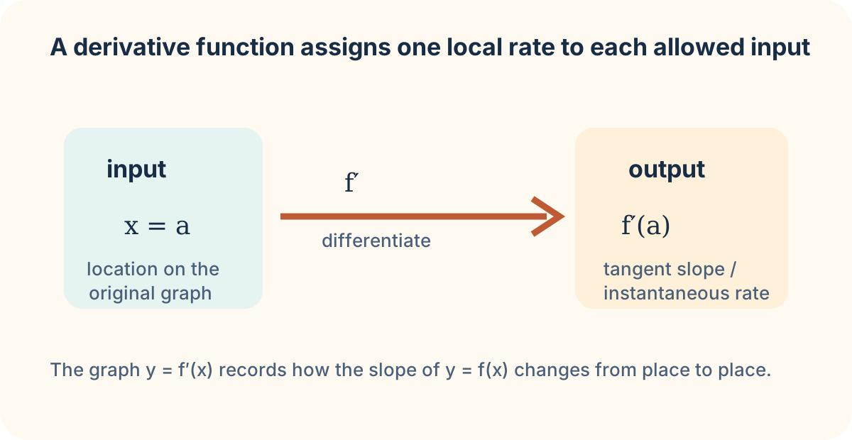
For $f(x)=x^2$, the derivative function is $f'(x)=2x$. This statement contains many individual derivative values. It says $f'(3)=6$, $f'(0)=0$, and $f'(-2)=-4$. The original function’s output at $x=-2$ is $4$, while its derivative’s output there is $-4$. One value is a height on the parabola; the other is the slope of the tangent line at that height. Keep the functions and their units separate.

Several notations can name the same derivative function. If $y=f(x)$, then $f'(x)$ and $\frac{dy}{dx}$ both refer to the derivative as a function of $x$. The Leibniz notation $\frac{dy}{dx}$ suggests a rate of output change per input change, which is useful in applied settings. It is not an ordinary fraction in the definition, although later methods can use its rate structure carefully. State the underlying functions before manipulating notation.

Read the signs of the derivative

If $f'(x)>0$ over an interval, tangent slopes are positive there, and $f$ is increasing on that interval. If $f'(x)<0$, tangent slopes are negative, and $f$ is decreasing. If $f'(a)=0$, the tangent line at $a$ is horizontal. That zero is a candidate for a local maximum, local minimum, or neither; later lessons provide tests for deciding which.

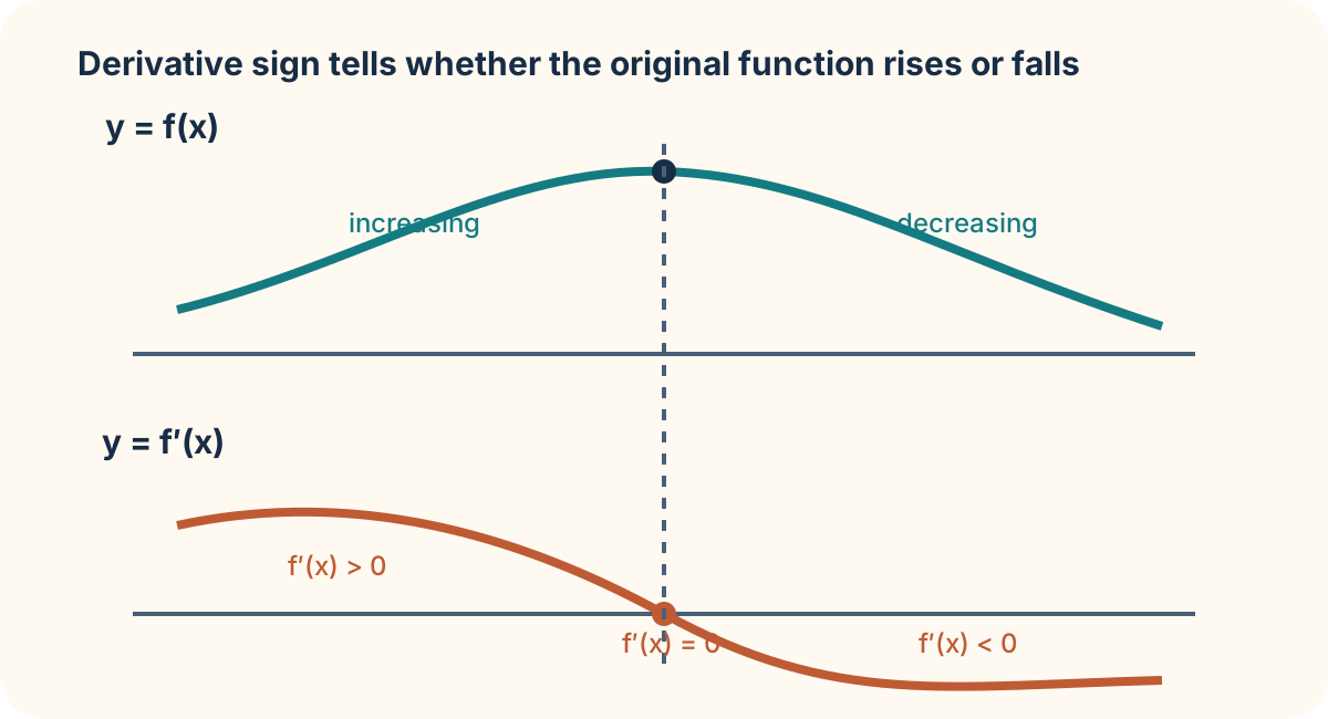
This interpretation works in reverse too. A graph of $f'$ above the horizontal axis records positive slopes of $f$. A graph of $f'$ below the axis records negative slopes of $f$. Where the derivative graph crosses or touches zero, the original graph has a horizontal tangent if it is differentiable there. The original graph need not cross its own axis at those same inputs; zeros of $f$ and zeros of $f'$ answer different questions.

For example, the function $f(x)=x^2$ has $f'(x)=2x$. The derivative is negative for $x<0$, so the parabola decreases as inputs move rightward toward zero. It is positive for $x>0$, so the parabola increases after zero. At $x=0$, $f'(0)=0$, matching the horizontal tangent at the parabola’s minimum. The sign change from negative to positive is the evidence for a minimum, not merely the fact that the derivative equals zero.

Estimate a local rate from a table

Experiments often supply values in a table rather than a formula. We cannot take a literal limit from finitely many measurements, but we can estimate a derivative using average rates over short intervals. When readings exist on both sides of the target, a centered difference compares symmetric nearby values:

$$f'(a)\approx\frac{f(a+h)-f(a-h)}{2h}.$$

The approximation improves only when the data are sufficiently accurate and the function is appropriately smooth over the selected scale. Smaller intervals can magnify measurement noise, so “closer” is not automatically better for experimental data.

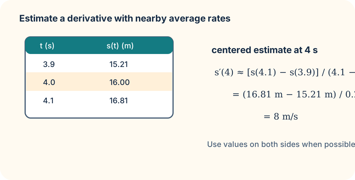
Suppose a temperature is recorded as $18.2\,\mathrm{^{\circ}C}$ at $9\,\mathrm{min}$ and $19.0\,\mathrm{^{\circ}C}$ at $11\,\mathrm{min}$. A centered estimate at $10\,\mathrm{min}$ is

$$T'(10)\approx\frac{19.0\,\mathrm{^{\circ}C}-18.2\,\mathrm{^{\circ}C}}{11\,\mathrm{min}-9\,\mathrm{min}} =0.4\,\frac{\mathrm{^{\circ}C}}{\mathrm{min}}.$$

The result says the temperature is increasing at roughly $0.4\,\frac{\mathrm{^{\circ}C}}{\mathrm{min}}$ near ten minutes. It does not say that the temperature itself is $0.4\,\mathrm{^{\circ}C}$. Units guard against that mistake.

Domain and common interpretation errors

Do not assume that a derivative exists wherever a function is defined. For $f(x)=|x|$, $f(0)=0$ but the derivative does not exist at zero because the one-sided slopes differ. For $f(x)=\sqrt{x}$, the domain begins at zero and the right-hand behavior at zero is special; there is no two-sided interior derivative in the usual sense. A derivative function inherits constraints from both the original domain and the local slope limit.

Another error is to confuse a large function value with a large derivative. A mountain can be high but flat at its summit, giving a large height and derivative zero. A low, steep path can have a small height and a large positive derivative. The derivative measures local change, not amount. In applications, this is the difference between a total inventory and its rate of accumulation, or between position and velocity.

Finally, a derivative value is local rather than a promise about a whole interval. If $f'(2)=5$, then near $x=2$ the function increases by about five output units per input unit. It does not guarantee a constant slope of five farther away. The next lesson develops rules that calculate derivative functions efficiently, but retain this local interpretation as a check on every symbolic answer.