Derivative as Instantaneous Rate and Tangent Slope

Calculus began with an apparently impossible request: find a rate at one instant rather than across an interval. Dividing a change in position by a nonzero change in time gives an average velocity, not a velocity at one chosen instant. Dividing by zero would destroy the calculation. The derivative resolves this tension by computing ordinary average rates over shrinking intervals and then asking whether their values approach one stable number. That limiting value is the instantaneous rate.

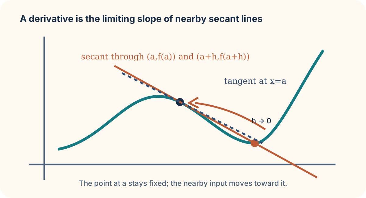
The same construction has a geometric interpretation. A secant line crosses a graph at two points, so its slope records average change between two inputs. Hold one point fixed and let the other slide toward it. If the secant slopes settle, their limit is the tangent slope at the fixed point. The derivative is therefore not two unrelated ideas—one physical and one geometric—but one limit interpreted in two contexts.

By the end, you should write and read the derivative definition, explain every part of the difference quotient, and attach meaningful units to a derivative. You should also know why the nearby point must remain distinct until after the average-rate calculation is formed. The next lesson will organize derivative values into a new function. For now, the focus is meaning before computation.

Start with a genuine average rate

For a function $f$, compare the outputs at $a$ and $a+h$. The symbol $h$ is an input change, so $a+h$ is a nearby input when $h$ is small. The resulting average rate is

$$\frac{f(a+h)-f(a)}{h}, \qquad h\ne0.$$

The numerator $f(a+h)-f(a)$ is output change. The denominator $(a+h)-a=h$ is input change. The restriction $h\ne0$ is essential at this stage because the quotient divides by $h$. It is an ordinary, valid secant slope for every permitted nonzero $h$.

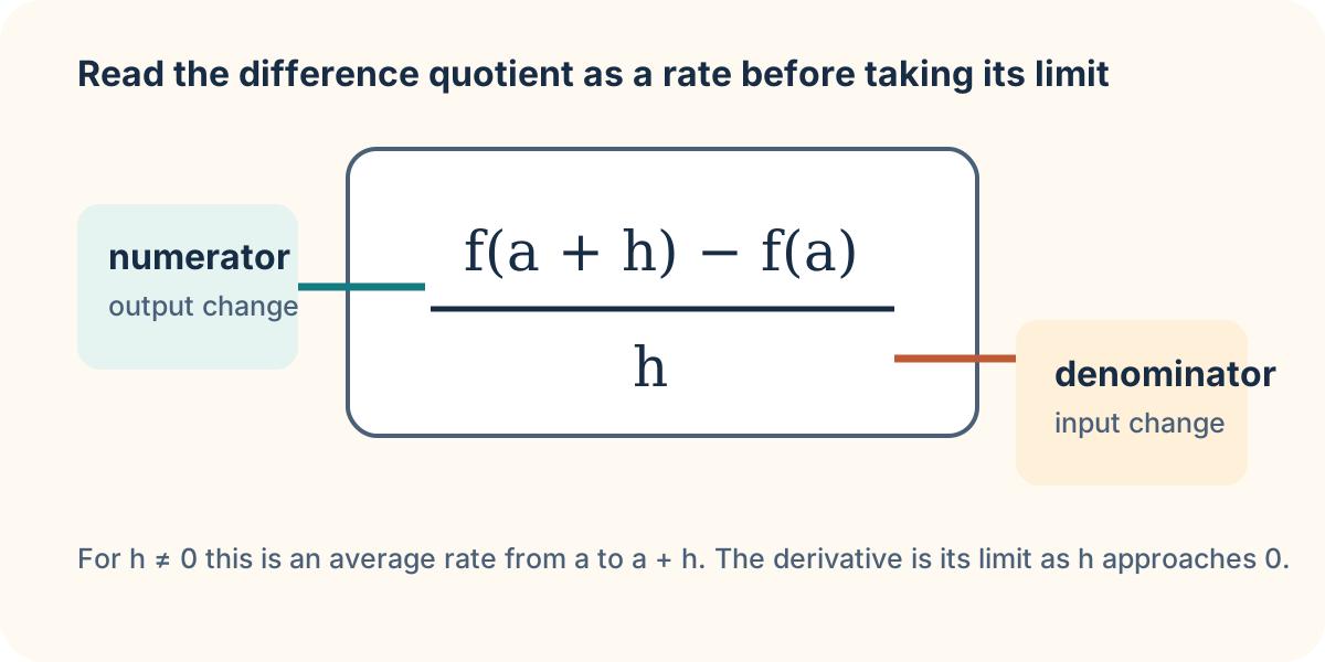
The derivative at $a$ is the limit of these average rates, when the limit exists:

$$f'(a)=\lim_{h\to0}\frac{f(a+h)-f(a)}{h}.$$

The prime is read “f prime.” It names a number: the local rate at the input $a$. The limit does not substitute $h=0$ into the fraction. Instead, it asks what the permitted quotient values approach as nonzero $h$ becomes arbitrarily small from both directions. This is exactly the nearby-versus-at distinction developed in the limits unit.

Secant slopes converge to a tangent slope

On the graph of $y=f(x)$, the two points $(a,f(a))$ and $(a+h,f(a+h))$ determine a secant line. Its slope is the difference quotient. As $h$ approaches zero, the second point moves toward the first. If the secant lines approach one stable line, that limiting line is tangent to the graph at $x=a$, and its slope is $f'(a)$.

For $f(x)=x^2$ at $a=3$, calculate before taking the limit:

$$\frac{(3+h)^2-3^2}{h} =\frac{6h+h^2}{h} =6+h.$$

The cancellation is valid only while $h\ne0$, which is already part of the quotient’s domain. Now the expression $6+h$ has limit six as $h$ approaches zero. Therefore $f'(3)=6$. The parabola’s tangent line at $(3,9)$ has slope six; the same result is the instantaneous rate at which the output $x^2$ changes per unit input near three.

Units reveal what the derivative measures

If $s(t)$ is position measured in meters and $t$ is time measured in seconds, then the quotient

$$\frac{s(t+h)-s(t)}{h}$$

has units of $\frac{\mathrm{m}}{\mathrm{s}}$. Its limiting value $s'(t)$ has the same units. We call it velocity. The units are not decorative: they tell us that the derivative compares position change to time change. If a temperature $T$ is measured in degrees Celsius as a function of time in minutes, then $T'(t)$ has units $\frac{\mathrm{^{\circ}C}}{\mathrm{min}}$.

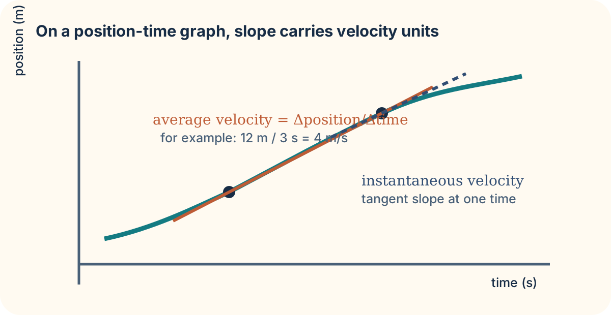
Suppose a vehicle’s position model is $s(t)=4t^2$, where $s$ is in meters and $t$ is in seconds. At $t=2\,\mathrm{s}$, the derivative will be $16\,\frac{\mathrm{m}}{\mathrm{s}}$. That number does not say the vehicle is sixteen meters from the origin; it says position is increasing by approximately sixteen meters for each additional second at that instant. A derivative’s numerical value is inseparable from its output-per-input units.

Rates can be negative, zero, or positive. A negative velocity means the position coordinate decreases as time increases; it does not necessarily mean an object slows down. A zero derivative means a horizontal tangent or instantaneously unchanged output, but a later lesson will show that it need not be a maximum or minimum. Interpret the sign in the model’s coordinate system before importing ordinary-language assumptions.

When the derivative does not exist

The derivative fails at a point if the secant slopes do not approach one finite common value. At a corner such as $f(x)=|x|$ at zero, slopes from the left approach $-1$ and slopes from the right approach $1$. The function is continuous there, but the directional rates disagree. A cusp, a vertical tangent, or a discontinuity can also prevent an ordinary finite derivative.

This explains why a graph may have a point but no tangent slope. Continuity asks whether nearby heights agree with the assigned height. Differentiability asks the more demanding question of whether nearby slopes agree with one another. When the latter succeeds, the derivative offers a linear local description: very close to $a$, the function changes approximately as its tangent line changes. That approximation will become explicit in the applications unit.

Before applying shortcut rules, practice translating each notation. The expressions $f'(a)$, $\frac{dy}{dx}\big|_{x=a}$, and “the slope of the tangent at $x=a$” name the same local-rate value when a derivative exists. Keep the evaluation point visible. The next lesson shifts from one value $f'(a)$ to the full derivative function $f'(x)$, whose input is a location and whose output is a local rate.