Higher Derivatives and Motion

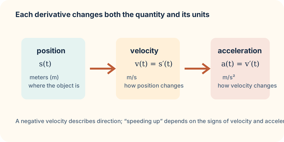
The derivative of a function is itself a function, so it can be differentiated again. Higher derivatives describe how rates change. In a motion model, position differentiates to velocity, and velocity differentiates to acceleration. This sequence is a model of linked quantities, not merely an exercise in adding prime marks. Units and signs tell us what each derivative means.

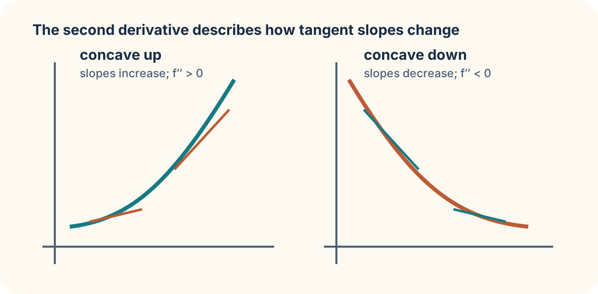
The second derivative also supplies geometric information. It measures how tangent slopes change as the input changes. Positive second derivative means slopes are increasing and the graph bends upward; negative second derivative means slopes are decreasing and the graph bends downward. This local shape information will later support graph analysis and optimization.

By the end, you should distinguish position, velocity, and acceleration by both definition and units; decide whether an object speeds up or slows down from signs; and connect the sign of a second derivative to concavity. Each interpretation begins with the function being modeled. Do not attach motion language to a derivative unless the original variables justify it.

The derivative ladder in a motion model

Let $s(t)$ be position in meters at time $t$ in seconds. Velocity is

$$v(t)=s'(t),$$

so its units are $\frac{\mathrm{m}}{\mathrm{s}}$. Acceleration is

$$a(t)=v'(t)=s''(t),$$

with units $\frac{\mathrm{m}}{\mathrm{s}^2}$. Each derivative divides by another time unit. Saying acceleration is “meters per second squared” means velocity changes by a certain number of meters per second during each second, not that distance itself is squared.

If $s(t)=t^3-6t^2+9t$ in meters, then $v(t)=3t^2-12t+9$ in $\frac{\mathrm{m}}{\mathrm{s}}$, and $a(t)=6t-12$ in $\frac{\mathrm{m}}{\mathrm{s}^2}$. At $t=1\,\mathrm{s}$, velocity is $0\,\frac{\mathrm{m}}{\mathrm{s}}$ while acceleration is $-6\,\frac{\mathrm{m}}{\mathrm{s}^2}$. The object is momentarily at rest but not necessarily stopped forever; its velocity is changing in the negative direction.

Direction and speed are different questions

Velocity sign indicates direction in the chosen coordinate system. Positive velocity means position increases; negative velocity means position decreases. Speed is $|v(t)|$, so it ignores direction. An object speeds up when speed increases and slows down when speed decreases. To determine this from signs, compare velocity and acceleration.

When $v$ and $a$ have the same sign, velocity moves farther from zero in its current direction, so speed increases. When they have opposite signs, velocity moves toward zero, so speed decreases. For example, $v=-4\,\frac{\mathrm{m}}{\mathrm{s}}$ and $a=-2\,\frac{\mathrm{m}}{\mathrm{s}^2}$ mean the object travels in the negative direction and is speeding up. A negative acceleration does not automatically mean slowing down.

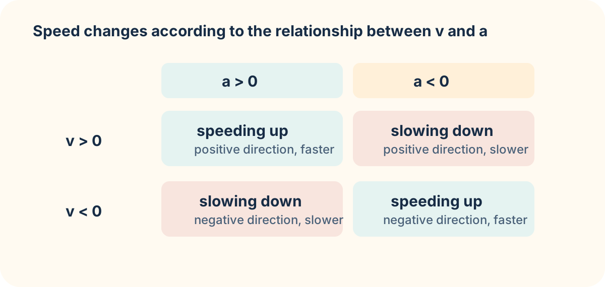
This sign logic is more reliable than ordinary-language intuition. State the interval, determine the sign of each function there, then interpret their relationship. At a time where velocity is zero, classify the behavior using signs on either side instead of relying only on the one instant. A direction change occurs when velocity changes sign, not merely when acceleration is zero.

Second derivative and concavity

For a general function $f$, the second derivative $f''$ describes how the first derivative changes. If $f''(x)>0$ on an interval, tangent slopes increase as $x$ increases, and the graph is concave up. If $f''(x)<0$, tangent slopes decrease, and the graph is concave down. Concavity concerns bending, not whether the function’s values are positive or negative.

For $f(x)=x^3$, $f'(x)=3x^2$ and $f''(x)=6x$. The graph is concave down when $x<0$ and concave up when $x>0$. At $x=0$, the second derivative is zero and concavity changes, so the point is an inflection point. A zero second derivative alone is only a candidate; the sign must actually change across the point.

In a position model, positive acceleration tells us velocity increases, which mirrors concave-up position. Negative acceleration tells us velocity decreases, which mirrors concave-down position. The same derivative structure supports both graph language and physical interpretation. Units add the physical meaning when the variables represent motion.

Prepare for optimization and graph analysis

Before solving an application, make a chain of labeled quantities. For a position function, label $s$, $v=s'$, and $a=s''$ with units. For a generic graph, label $f$, slope $f'$, and slope-change $f''$. Then create a sign chart that divides the domain at values where the relevant derivative is zero or undefined. This organization makes later optimization and curve-sketching arguments transparent.

Practice with $s(t)=2t^3-9t^2+12t$ in meters. Find velocity and acceleration, then identify times when the particle is at rest and intervals where it speeds up or slows down. State every conclusion with units and an interval. Next, use $f''$ to determine concavity for $f(x)=x^4-4x^2$. The next lesson asks a related question: when a derivative vanishes or fails, which points can be maxima or minima under a stated domain?