One-Sided Limit Notation and Direction

A two-sided limit compresses two approach directions into one statement. At a jump, endpoint, or vertical asymptote, that compression can hide the most important behavior. One-sided limits expose the left and right approaches separately. Their superscripts describe where input values lie relative to the target, not whether the inputs or outputs are positive or negative. Direction belongs first to the input domain.

This lesson develops left-hand and right-hand notation through number lines, graphs, tables, and piecewise formulas. We will translate each symbol into a complete sentence and distinguish input direction from output direction. We will also decide which side of a piecewise rule governs nearby values. The guiding question is: what exactly is being restricted when a limit is taken from one side? The next lesson combines the directional statements into the two-sided existence criterion.

By the end, you should read $\lim_{x\to a^-}f(x)$ and $\lim_{x\to a^+}f(x)$ accurately, create directional tables, and choose the correct piecewise branch. You should explain why the superscripts are not signs of the limit value. You should identify the available approach at a domain endpoint. You should also state a directional conclusion without relying on vague phrases such as “from that side.” Precision here prevents later existence errors.

The superscript locates the moving input

The notation

$$\lim_{x\to a^-}f(x)=L$$

means that outputs approach $L$ as $x$ approaches $a$ through values less than $a$. The minus superscript is read “from the left.” It does not mean that $x$ must be negative, that the outputs are negative, or that a quantity is being subtracted. For $a=5$, the values $4.9$, $4.99$, and $4.999$ approach from the left even though they are positive.

The notation

$$\lim_{x\to a^+}f(x)=L$$

uses inputs greater than $a$ and is read “from the right.” Values $5.1$, $5.01$, and $5.001$ approach five from that side. Their outputs may approach $L$ from above, below, or by alternating around it. Input direction and output direction are independent. The superscript modifies the input approach.

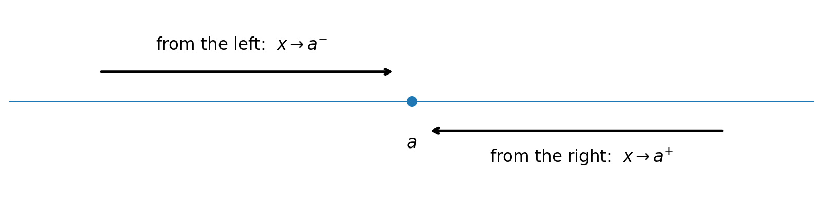
The ordinary notation $\lim_{x\to a}f(x)$ carries no superscript because it asks for one destination across every locally available direction. A one-sided claim is weaker because it restricts the allowed nearby inputs. It can exist when the ordinary limit does not. One-sided notation does not repair behavior; it describes a smaller approach set. That smaller set must still stabilize.

Directional tables make the restriction visible

A left-hand table lists inputs less than the target and moves them closer. For $a=2$, values might be $1.9$, $1.99$, and $1.999$. A right-hand table uses $2.1$, $2.01$, and $2.001$. Place the two groups in separate columns rather than sorting all inputs into one sequence. The organization should display the mathematical question.

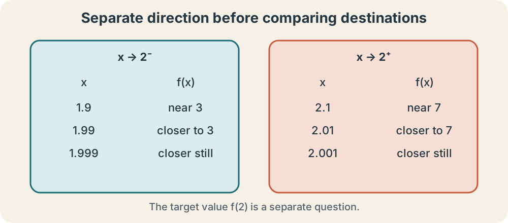
Suppose a table shows left-side outputs approaching three and right-side outputs approaching seven. The left-hand limit is three and the right-hand limit is seven, based on the displayed evidence. Neither conclusion determines $f(2)$. A row at $x=2$ answers a point-value question and should be recorded separately. The table can support both one-sided statements even though the destinations disagree.

Finite rows remain evidence rather than proof. An oscillating function can behave unexpectedly between selected inputs on one side. Increasing sample density may reveal trouble but cannot exhaust every closer value. Algebraic structure or a theorem supplies stronger control. Directional organization improves the evidence without changing its logical status.

Read direction from a graph

To read the left-hand limit, begin on the graph at inputs smaller than $a$ and trace toward the target. To read the right-hand limit, begin at larger inputs and trace toward it. Watch the output height approached, ignoring the target’s filled point until the nearby behavior is recorded. The physical motion of a finger is only a reading aid. The mathematics concerns ordered domain values.

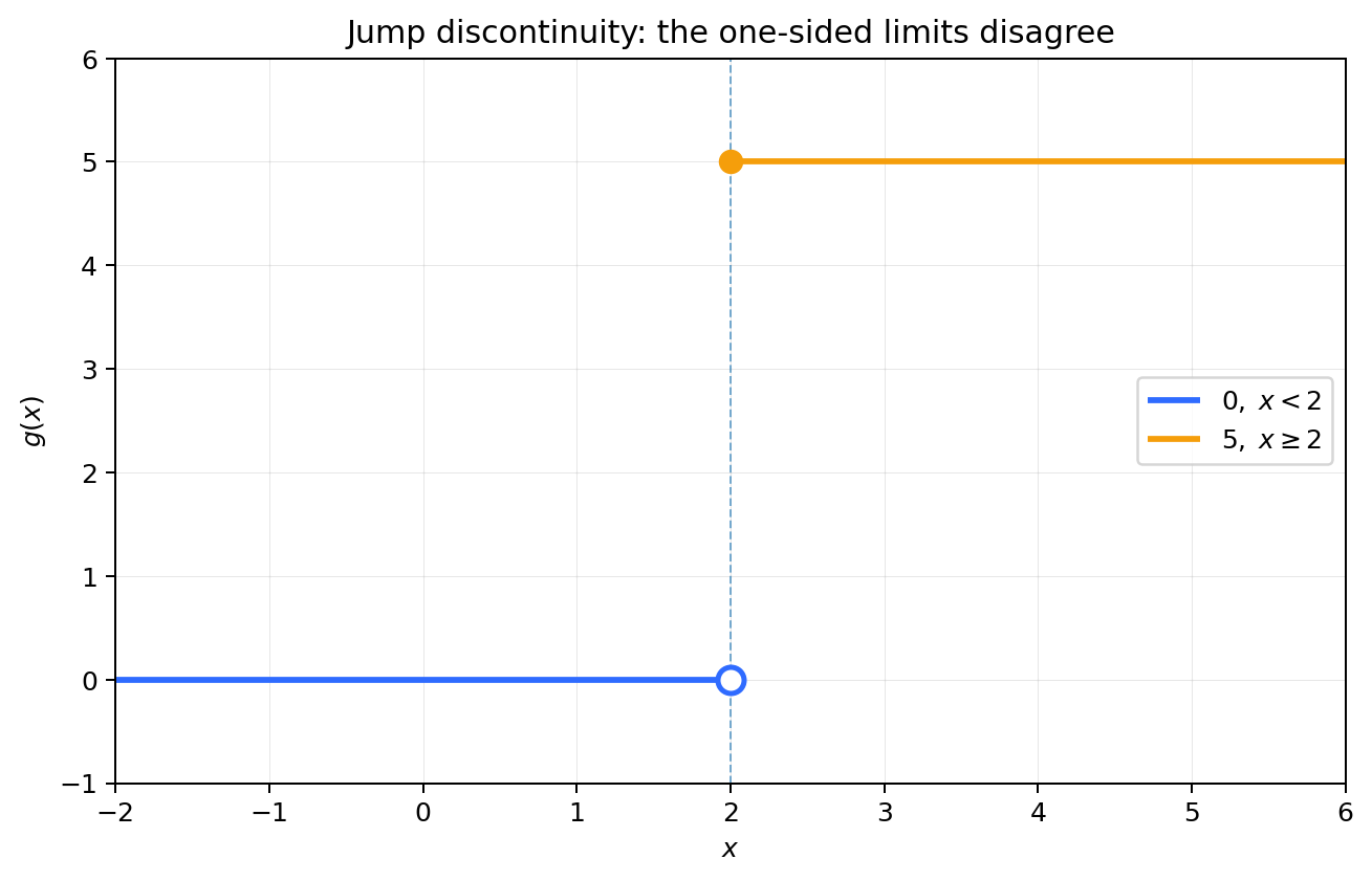
At a jump, each branch can approach a stable finite height. The graph therefore supports two one-sided limits even though the heights differ. A filled point on either branch or at a third height does not change either directional destination. Point assignment and directional behavior remain separate. The next lesson will explain why the mismatch defeats an ordinary limit.

Graph windows can create false endpoints. A branch ending at the screen edge may continue beyond the visible region. Consult the stated domain and arrows rather than treating the frame as mathematical evidence. Similarly, a rough graph may conceal a tiny gap or oscillation. Directional reading is only as precise as the representation permits.

Piecewise formulas require branch discipline

Consider

$$f(x)= \begin{cases} 2x+1, & x<3,\\ x^2-2, & x\ge3. \end{cases}$$

For the left-hand limit at three, nearby inputs satisfy $x<3$, so the first formula applies and approaches seven. For the right-hand limit, nearby inputs satisfy $x>3$, so the second formula applies and also approaches seven. Branch selection follows the direction of nearby inputs.

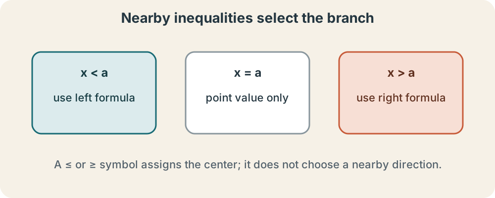
The equality attached to $x\ge3$ determines the point value, not the right-hand limit. Replacing it with $x>3$ and defining $f(3)=100$ elsewhere would leave both directional limits unchanged. Only nearby values on the proper side matter. This distinction is especially useful in parameter problems where continuity is enforced. First find directional destinations, then address the point.

If the left formula approaches $2k+1$ and the right formula approaches seven, matching directions requires $2k+1=7$. Solving gives $k=3$. The equation comes after the conceptual branch analysis. Substituting into whichever formula happens to contain an equality sign can solve the wrong problem. Inequalities govern approach; equality governs assignment.

Domain endpoints permit only available directions

For $g(x)=\sqrt{x}$ on its real domain, no allowed inputs lie immediately left of zero. The meaningful endpoint statement is

$$\lim_{x\to0^+}\sqrt{x}=0.$$

Demanding a real left-hand approach would invent inputs outside the domain. Limits are always relative to the function’s domain.

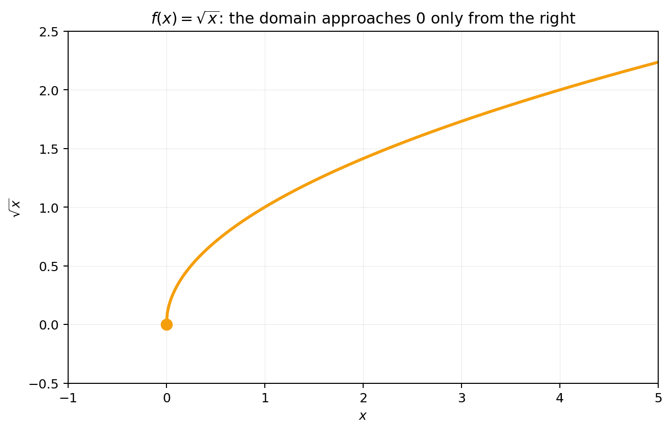
Many continuity conventions use the available one-sided limit at an endpoint. This is not an arbitrary exception. A time model beginning at $t=0\,\mathrm{s}$ may have meaningful behavior immediately after the start without defining negative time. The same principle applies to inverse trigonometric domains and physical constraints. Domain analysis determines the required directions.

At an interior point, both sides ordinarily contain allowed inputs and should be checked. At a boundary, identify the locally available side before making a claim. At an isolated domain point, there may be no surrounding inputs from either side, so ordinary nearby-limit language requires additional convention or is inapplicable. The domain is not a footnote. It determines the approach paths.

Synthesis and transition

For the piecewise function above, create two directional tables near three and verify the symbolic conclusions. Then change the right branch to $x^2+1$ and repeat. State both one-sided limits and the point value in complete sentences. Explain which change affects nearby behavior and which inequality determines the point. Do not yet collapse the directions into an ordinary limit.

Next sketch a function with left-hand limit $-2$, right-hand limit $4$, and point value $10$ at $x=1$. Label the relevant open and filled points. Write all three symbolic statements. Then create an endpoint example that supports only a left-hand approach. State its domain explicitly and explain why the missing direction is not a failure.

One-sided limit notation restricts the moving input to values below or above a target. The superscripts encode position in input space, while the limiting value records a destination in output space. Tables, graphs, and piecewise formulas should preserve that distinction. Domain endpoints show that direction requirements come from available inputs. The next lesson asks when the separate directional claims combine into one ordinary limit.