Infinite Limits and Limits at Infinity

Finite limits describe outputs settling near a real number. Some functions do not settle near any finite height. Their magnitudes can grow beyond every chosen bound as an input approaches a finite target or as inputs travel indefinitely far. Infinity notation describes this unbounded behavior compactly. It does not name a real output attained by the function.

This lesson separates two questions that are often confused. An infinite limit concerns what happens near a finite input such as $x=0$. A limit at infinity concerns what happens as $x$ becomes arbitrarily large in magnitude. We will interpret directional signs, identify vertical and horizontal asymptotes, and compare rational end behavior by degrees. The guiding question is: which quantity is approaching infinity, and what does that claim actually mean?

By the end, you should read all four common infinity-limit forms, distinguish vertical from horizontal asymptotes, and analyze basic rational functions. You should explain why infinity is not a number that can be substituted. You should also keep left- and right-hand behavior separate when signs differ. The next lesson returns to finite limits through continuity and the Intermediate Value Theorem.

Unbounded behavior near a finite target

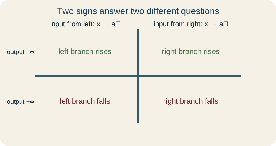
For $f(x)=\frac1x$, inputs can approach zero without ever equaling zero. Positive inputs produce increasingly large positive outputs, while negative inputs produce increasingly large negative outputs. We write

$$\lim_{x\to0^+}\frac1x=+\infty, \qquad \lim_{x\to0^-}\frac1x=-\infty.$$

The superscript identifies the input direction, while the infinity sign describes the output’s unbounded sign.

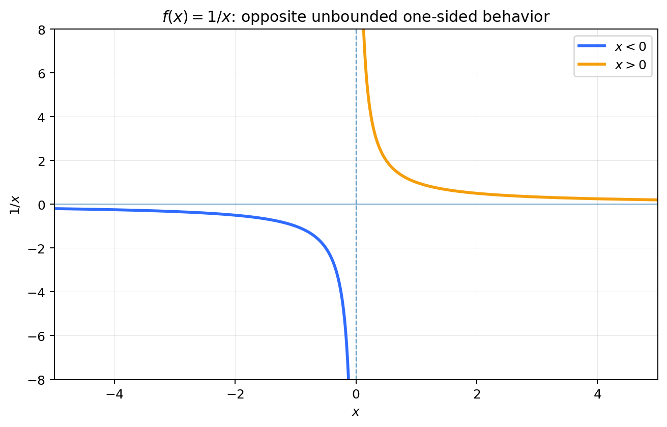
The statement $\lim_{x\to0^+}\frac1x=+\infty$ means that for every positive height $B$, outputs eventually exceed $B$ when positive inputs are sufficiently close to zero. It does not mean that $\frac1x$ equals infinity at zero. The function is undefined there. Unboundedness is behavior near the target, not a point value.

Because the two directional behaviors have opposite signs, there is no common two-sided infinite statement of one sign. Saying merely “the limit does not exist” is correct but incomplete. The directional notation explains why. A vertical asymptote at $x=0$ records the graph’s unbounded behavior, not a vertical line that the function becomes.

Signs come from factored nearby structure

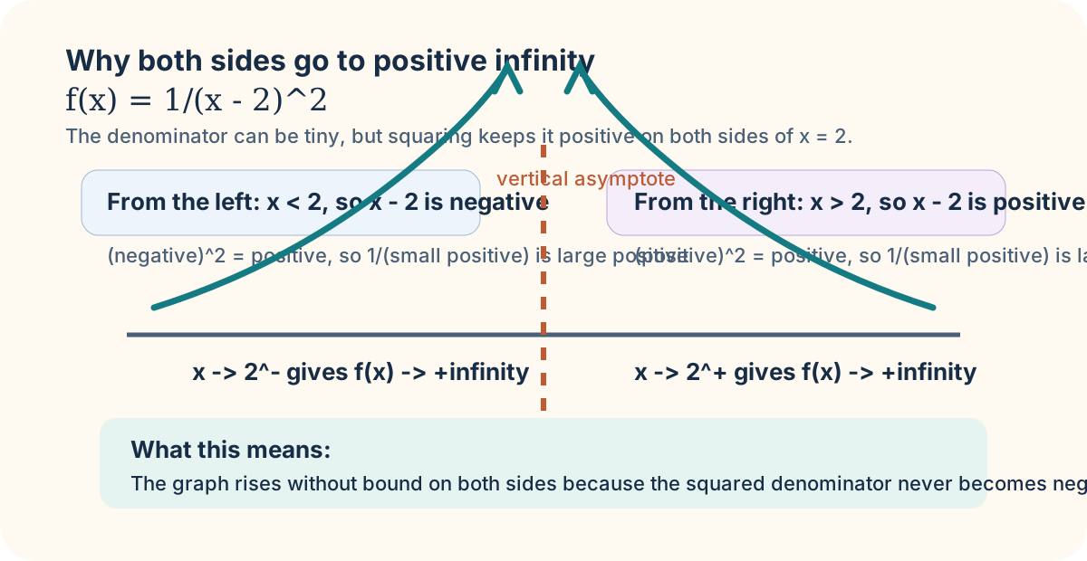
For $\frac1{(x-2)^2}$, the denominator is positive on both sides of two and approaches zero through positive values. Thus both directional outputs grow positively, and

$$\lim_{x\to2^-}\frac1{(x-2)^2}=+\infty, \qquad \lim_{x\to2^+}\frac1{(x-2)^2}=+\infty.$$

The even power preserves sign. A two-sided extended statement may therefore use $+\infty$ by convention.

For $\frac{x+1}{(x-2)^3}$, the numerator stays positive near two while the odd-power denominator changes sign. The left side approaches negative infinity and the right side approaches positive infinity. Factored forms and simple sign charts are safer than graph guessing. They reveal which factors change sign and which stay bounded away from zero.

Cancellation must be completed before classifying a potential asymptote. The expression $\frac{x^2-4}{x-2}$ has an apparent zero denominator at two, but factoring cancels the common factor nearby and produces a removable hole, not a vertical asymptote. An infinite-limit conclusion requires an uncancelled denominator factor approaching zero while the remaining quotient stays nonzero or unbounded in the appropriate way.

Limits at infinity ask a different question

The notation

$$\lim_{x\to\infty}f(x)=L$$

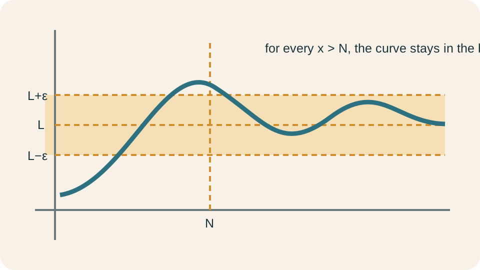
asks what outputs approach as inputs become arbitrarily large and positive. The notation $x\to-\infty$ asks the corresponding question for large negative inputs. No finite target input is involved. A graph may approach a horizontal asymptote $y=L$ without ever reaching it.

For $f(x)=\frac1x$, both $\lim_{x\to\infty}f(x)=0$ and $\lim_{x\to-\infty}f(x)=0$. The outputs approach zero from positive and negative sides respectively. The vertical asymptote at zero and horizontal asymptote at zero concern different input behavior. One occurs near a finite input; the other occurs far away. They should never be conflated.

Long-run limits often describe model saturation, decay, or baseline behavior. If a concentration model approaches $2\,\frac{\mathrm{mg}}{\mathrm{L}}$ as time grows, the statement concerns late times, not an impossible “time equals infinity.” The horizontal asymptote is a predictive tendency within the model’s assumptions. Context still limits extrapolation.

Compare rational functions by degree

For a rational function $\frac{p(x)}{q(x)}$, the leading terms determine behavior as $|x|$ becomes large. If the degree of the numerator is less than the degree of the denominator, the limit at both positive and negative infinity is zero. For example, $\frac{3x+1}{x^2-4}\to0$. Lower-degree terms become negligible compared with the dominant denominator power.

If the degrees are equal, the long-run limit is the ratio of leading coefficients. Thus $\frac{5x^2-1}{2x^2+7}\to\frac52$. Dividing numerator and denominator by the highest power of $x$ makes this structure explicit. Terms containing inverse powers vanish as $|x|$ grows. The result is a horizontal asymptote when the rational function is defined sufficiently far out.

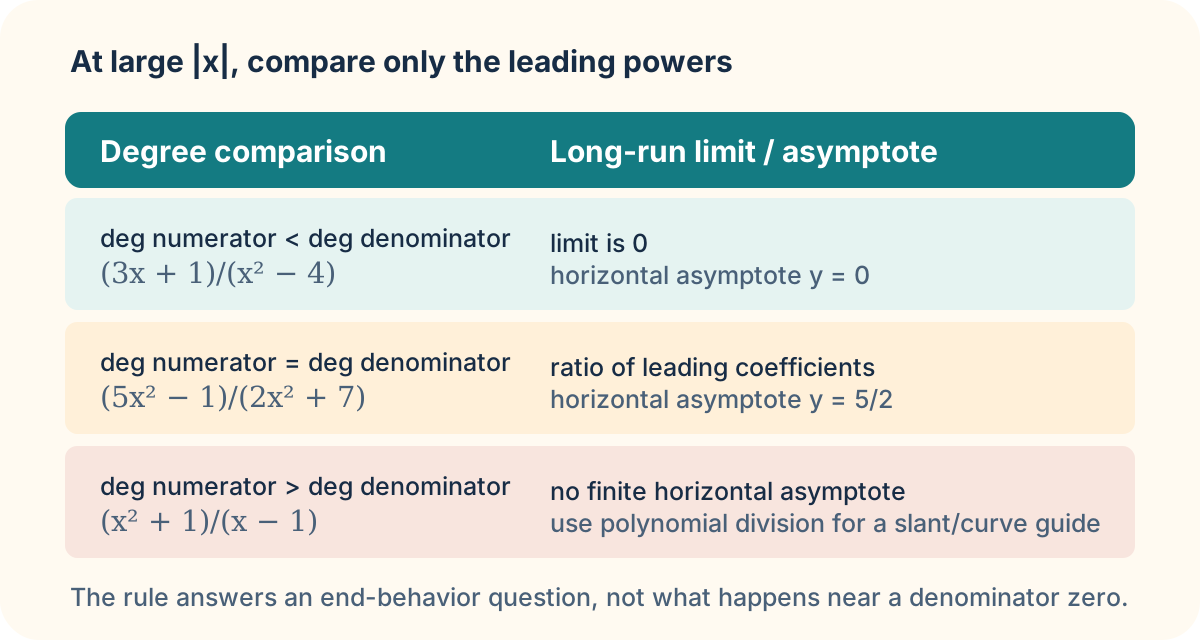
If the numerator degree exceeds the denominator degree, no finite horizontal asymptote follows from this rule. Polynomial division may reveal a slant or higher-degree asymptote. For $\frac{x^2+1}{x-1}$, division gives $x+1+\frac2{x-1}$, so the graph approaches the line $y=x+1$ at infinity. The next-order behavior matters.

Formal language changes the bound, not the logic

For a finite limit at infinity, the output tolerance is still epsilon, but the input condition becomes $x>N$ rather than $|x-a|<\delta$. The statement $\lim_{x\to\infty}f(x)=L$ means that for every $\varepsilon>0$, some threshold $N$ exists such that $x>N$ implies $|f(x)-L|<\varepsilon$. The input is controlled by going far enough right, not by staying close to a finite center.

For an infinite limit near a finite target, a height bound replaces epsilon. The claim $f(x)\to+\infty$ as $x\to a$ means every positive bound $B$ can eventually be exceeded by choosing $x$ sufficiently close to $a$ from the stated direction. The same control logic remains: a requested output condition receives a sufficient input condition. Only the requested condition differs.

These formal versions prevent imprecise phrases such as “x gets to infinity.” Infinity describes unbounded direction, not an endpoint in the ordinary real domain. A threshold $N$ can always be exceeded by a larger real input. Likewise, a height bound $B$ can always be exceeded in an unbounded-output limit. The quantifier structure expresses a never-ending process through finite tests.

Synthesis and transition

Analyze $\frac{2}{x-3}$, $\frac{2}{(x-3)^2}$, and $\frac{x+1}{(x-3)^3}$ near $x=3$. Use a sign chart to state each directional limit. Identify which graphs have opposite signs and which have the same sign on both sides. Explain why a vertical asymptote does not assign a function value at the target.

Then determine the limits at positive and negative infinity of $\frac{4x^2-x+1}{2x^2+3}$ and $\frac{3x+1}{x^2+1}$. State the degree comparison and horizontal asymptote. Contrast these statements with the behavior of the same expressions near any denominator zeros. Keep finite-target and far-away questions in different sentences.

Infinite limits describe unbounded outputs near a finite target, while limits at infinity describe long-run output behavior as inputs grow without bound. Directional signs, factor parity, and rational degrees organize the analysis. Infinity is notation for behavior, not an input or output value to substitute. The next lesson returns to functions that do have finite local behavior and asks when they are continuous enough to guarantee intermediate outputs. The Intermediate Value Theorem turns that continuity into an existence result.