Basic Derivative Rules

The derivative definition is the source of every differentiation rule, but re-expanding a difference quotient for every polynomial would be inefficient and obscure the structure we want to see. Basic rules package recurring limit arguments into reliable steps. They are not new definitions of derivative. They are consequences of the same local-rate limit, and they must be used only where their hypotheses fit the expression.

This lesson develops the rules for constants, sums and differences, constant multiples, and powers. These rules cover polynomial functions and many simple models. They do not yet handle a product of two changing factors, a quotient, or one function nested inside another. The next lesson introduces those cases deliberately, especially the Chain Rule, rather than treating every expression as though the power rule applies without thought.

By the end, you should be able to differentiate a polynomial term by term, explain the pattern in the power rule, and use the difference quotient to justify a simple rule. You should also recognize expressions that are not yet eligible for these rules alone. Efficient symbolic work is useful only when it remains attached to the function structure.

Linearity: constants, sums, and constant multiples

The derivative of a constant is zero:

$$\frac{d}{dx}(c)=0.$$

A constant function has the same output at every nearby input, so its output change is zero. Its secant and tangent slopes are both zero. For example, a temperature held at $22\,\mathrm{^{\circ}C}$ has rate of change $0\,\frac{\mathrm{^{\circ}C}}{\mathrm{min}}$ with respect to time, even though the temperature value itself is not zero.

Derivatives distribute across addition and subtraction:

$$\frac{d}{dx}[u(x)\pm v(x)]=u'(x)\pm v'(x).$$

They also preserve constant multipliers:

$$\frac{d}{dx}[c\,u(x)]=c\,u'(x).$$

Both facts follow because output changes add and constant factors can be pulled outside the difference quotient before taking a limit. A polynomial is a sum of constant multiples of powers, so these rules let us differentiate one term at a time.

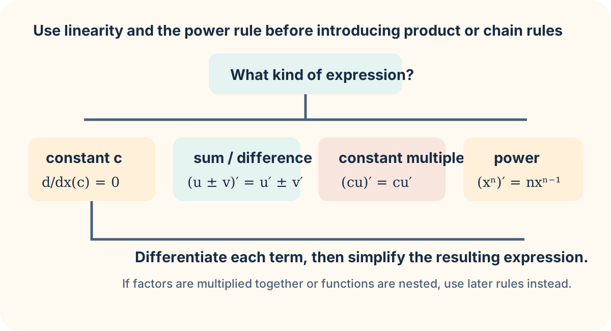
For instance, if $p(x)=5x^3-2x+7$, then differentiate each term: the constant multiple rule gives $15x^2$ for $5x^3$, the derivative of $-2x$ is $-2$, and the constant seven becomes zero. Thus $p'(x)=15x^2-2$. Preserve signs and coefficients while differentiating; the derivative of a sum is the sum of derivatives, not a reason to combine unlike terms incorrectly.

The power rule and its visible pattern

For a real exponent $n$ in a domain where the expression is defined, the power rule is

$$\frac{d}{dx}(x^n)=nx^{n-1}.$$

Read this in two moves: the old exponent becomes a coefficient, then the exponent decreases by one. For $x^4$, the derivative is $4x^3$. For $x$, understood as $x^1$, the derivative is $1x^0=1$. For a reciprocal written as $x^{-1}$, the derivative is $-x^{-2}$, which can be written $-\frac1{x^2}$ using a horizontal fraction bar.

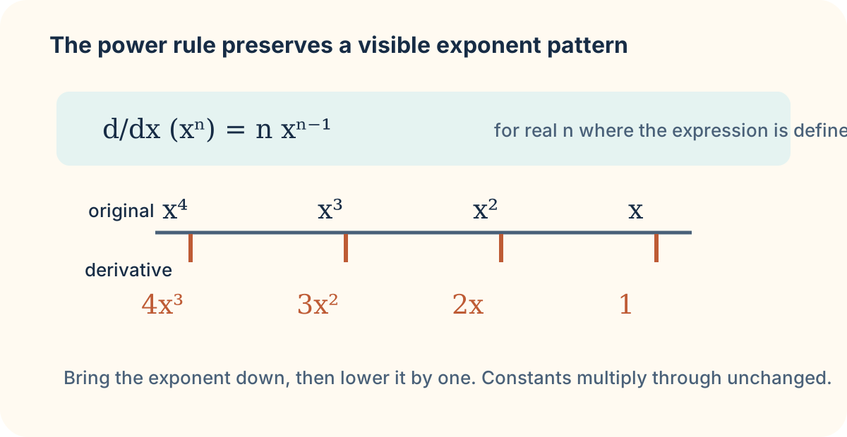
Do not misread the rule as “multiply by x.” The exponent changes, but the base stays $x$. The derivative of $x^5$ is $5x^4$, not $5x^6$ or $x^4$. Checking units and approximate behavior helps: a rapidly growing fifth-power function should have a rate that also grows rapidly for large positive $x$, as $5x^4$ does.

The rule works term by term in a polynomial. If $q(x)=3x^4-x^2+6$, then

$$q'(x)=12x^3-2x.$$

At $x=2$, this gives $q'(2)=92$. That is a slope or rate at input two, not the value $q(2)$. Keep evaluation as a final step when the question asks for one numerical derivative value.

See a rule emerge from the limit definition

For $f(x)=x^2$, start with the definition rather than the shortcut:

$$f'(x)=\lim_{h\to0}\frac{(x+h)^2-x^2}{h}.$$

Expanding produces $x^2+2xh+h^2-x^2$, so for nonzero $h$ the quotient becomes $2x+h$. Its limit as $h$ approaches zero is $2x$. This is the power rule for the special case $n=2$. Notice the order: form a quotient with $h\ne0$, simplify that legitimate expression, then take the limit.

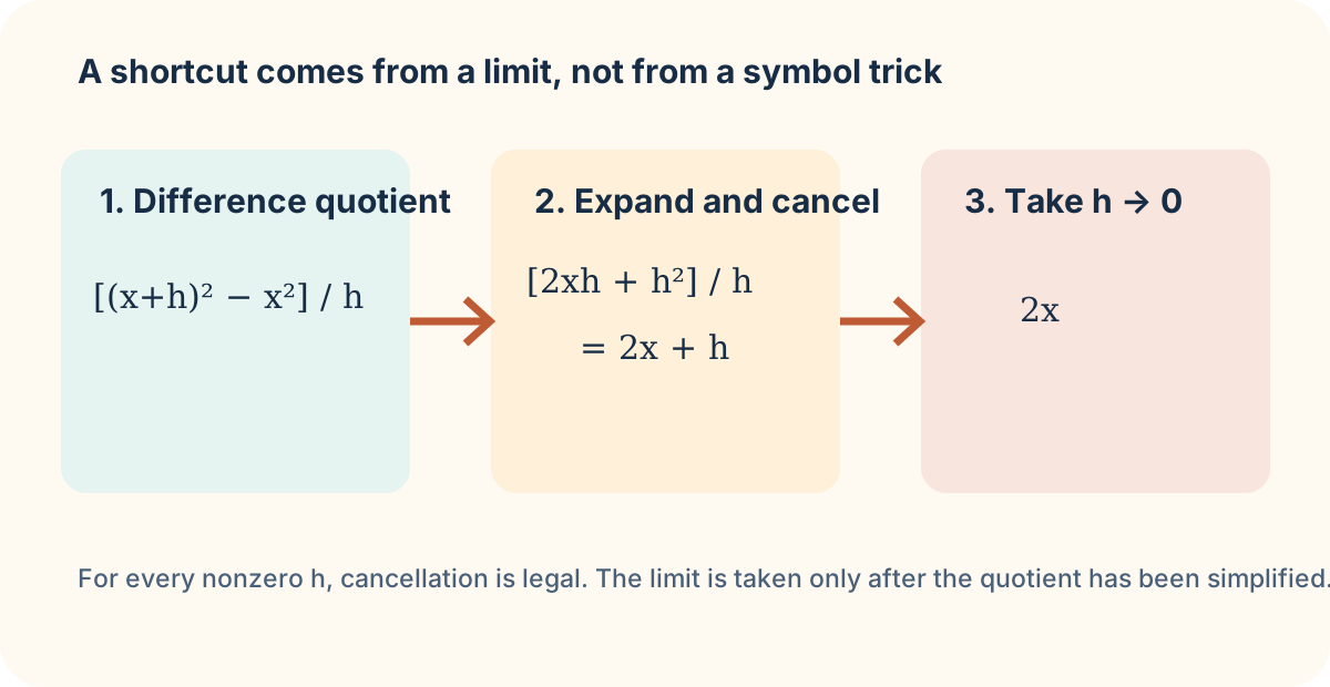
For a positive integer $n$, the expansion of $(x+h)^n$ contains a term $nx^{n-1}h$ plus terms with higher powers of $h$. Dividing by $h$ leaves $nx^{n-1}$ plus terms that contain $h$. Those remaining terms approach zero as $h$ approaches zero. A complete proof uses the binomial theorem, but the mechanism is already visible in the square case: one first-order change survives, while higher-order changes vanish in the local limit.

This derivation is worth remembering because it explains why the power rule has its particular shape. It is not simply a convention. It records the dominant first-order change in $x^n$ produced by a small input change. Later, linearization will use this same first-order idea to approximate functions.

Choose a rule that matches the structure

The basic rules apply cleanly to $7x^5-3x^2+4$. They do not justify differentiating $(x^2+1)^5$ as $5x^4$, because the base is not $x$ alone; it is a changing inner function. They also do not justify differentiating $x^2\sin x$ by treating it as one power. Those structures need the Chain Rule and Product Rule respectively.

Before differentiating, make a structural pass. Identify whether the expression is a sum of terms, a constant multiple, a power of $x$, a product, quotient, or composition. Apply only the rule that matches the outermost structure, and then simplify. This habit prevents most symbolic errors before they occur.

As preparation for the next lesson, differentiate $r(x)=4x^3-7x+2$ and evaluate $r'(2)$. Then compare the two expressions $(3x-1)^4$ and $x^4(3x-1)$. They look related, but one is a composition and the other is a product. Their derivatives require different rules. The next lesson develops those rules from this structural distinction.