Extreme Values and Optimization

Optimization asks for the best allowable value of a quantity, not merely a point where a derivative happens to be zero. A maximum or minimum depends on the objective and the domain. The derivative helps locate interior candidates, while endpoints and constraints remain part of the answer. A careful solution therefore begins with the question being optimized and ends by comparing actual objective values.

This lesson separates three ideas: local extrema, absolute extrema, and the modeling workflow for an applied optimization problem. The Extreme Value Theorem guarantees that a continuous function on a closed interval reaches an absolute maximum and minimum. The derivative then helps us find the finite list of locations worth checking. This combination of existence theorem and candidate test is the logical foundation for reliable optimization.

By the end, you should identify critical points, use the closed-interval method, apply the first derivative test, and construct a one-variable objective function from a constrained context. You should report a final answer with its units and domain, rather than ending at an untested derivative equation. The next lesson gives a theorem that relates an interval’s average change to an interior instantaneous rate.

Critical points are candidates, not conclusions

A critical point of $f$ is an interior domain value $c$ where $f'(c)=0$ or where $f'(c)$ does not exist while $f(c)$ does. Local maxima and minima can occur only at critical points under the usual differentiability assumptions, but not every critical point is an extremum. For example, $f(x)=x^3$ has $f'(0)=0$ but continues increasing through zero, so it has neither a local maximum nor a local minimum there.

The first derivative test checks behavior on either side of a critical point. If $f'$ changes from positive to negative, the function changes from increasing to decreasing, producing a local maximum. If $f'$ changes from negative to positive, it produces a local minimum. If the derivative sign does not change, the point may be flat without being extreme.

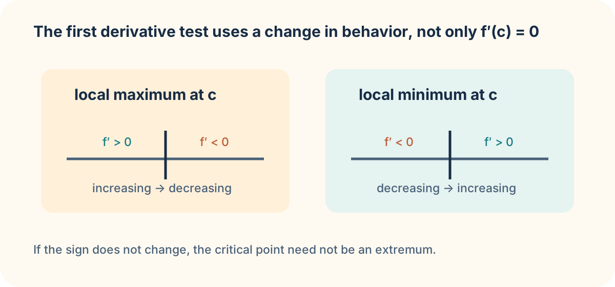
For $f(x)=x^3-3x$, the derivative is $f'(x)=3x^2-3$. Critical points occur at $x=-1$ and $x=1$. A sign chart shows positive derivative before $-1$, negative derivative between $-1$ and $1$, and positive derivative after $1$. Thus $x=-1$ is a local maximum and $x=1$ is a local minimum. The signs, not the equation $f'(x)=0$ alone, justify the classifications.

Absolute extrema on a closed interval

If a function is continuous on $[a,b]$, the Extreme Value Theorem says it has both an absolute maximum and an absolute minimum on that interval. To find them, evaluate the function at every interior critical point and both endpoints. Compare the resulting output values. The largest is the absolute maximum; the smallest is the absolute minimum.

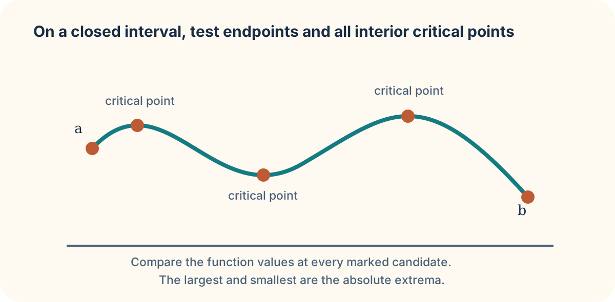
Suppose $f(x)=x^3-3x$ on $[-2,2]$. The candidates are $-2$, $-1$, $1$, and $2$. Their function values are $-2$, $2$, $-2$, and $2$, respectively. Thus the absolute maximum is $2$, reached at $x=-1$ and $x=2$, and the absolute minimum is $-2$, reached at $x=-2$ and $x=1$. An extremum may occur at more than one input.

The closed-interval procedure is different from finding local extrema on an unrestricted domain. Endpoints can be absolute extrema even though they are not interior critical points. If the domain is open or unbounded, an absolute maximum or minimum may fail to exist. State the domain before using a theorem or claiming “the maximum.”

Build an optimization model before differentiating

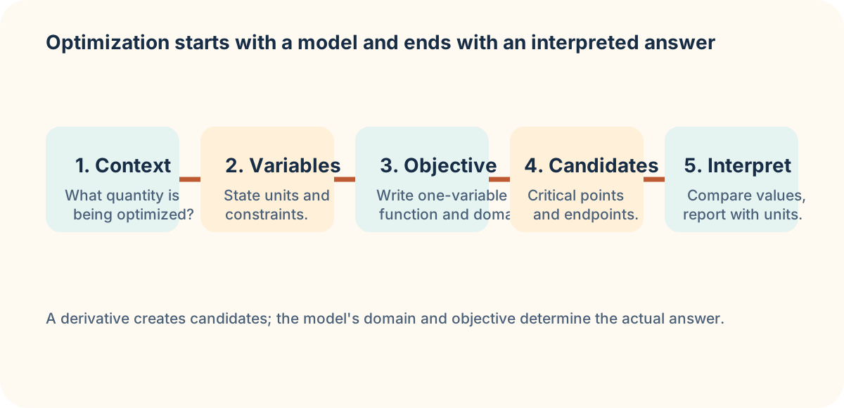
Applied optimization begins with context, variables, constraints, and one objective function. A rectangular enclosure with fixed perimeter, for example, has many width-length pairs. The perimeter condition lets one variable be eliminated, turning area into a function of one remaining variable. Differentiation comes after this modeling step, not before it.

If a rectangle has perimeter $40\,\mathrm{m}$, let width be $w\,\mathrm{m}$ and length be $(20-w)\,\mathrm{m}$. The area is

$$A(w)=w(20-w)=20w-w^2,$$

with domain $0\le w\le20$. The derivative is $A'(w)=20-2w$, giving a critical point at $w=10\,\mathrm{m}$. Comparing that candidate with the endpoints shows maximum area $100\,\mathrm{m}^2$ at a $10\,\mathrm{m}$ by $10\,\mathrm{m}$ square. The endpoints represent degenerate rectangles with zero area, so they must be checked even though the practical interpretation may exclude them.

Make conclusions match the question

An optimization response should name the optimized quantity, the input values that achieve it, the objective value, and units. “$w=10$” is incomplete if the question asks for maximum area. “The maximum is 100” is incomplete without square-meter units and the dimensions that achieve it. Also explain any context assumptions: nonnegative dimensions, a closed interval, or a continuous model.

Practice by maximizing the volume of an open-top box made from a square sheet after equal corner squares are removed. First define the cut size and its physical domain. Express volume as one function of that cut size, identify all closed-interval candidates, then compare volumes. The derivative will generate a candidate, but the domain and final comparison complete the proof. In the next lesson, the Mean Value Theorem will formalize another bridge between average and instantaneous rates.