Mean Value Theorem and Consequences

The Mean Value Theorem, or MVT, is a formal bridge between an interval-wide average rate and a local instantaneous rate. It says that a sufficiently well-behaved function has at least one interior point where the tangent slope matches the secant slope across the entire interval. The statement makes precise a common intuition: during a trip with a certain average velocity, there is some moment at which instantaneous velocity equals that average.

The theorem is conditional. Continuity on the closed interval and differentiability on the open interval are not ceremonial phrases; they prevent a function from jumping, breaking, or turning through a corner in a way that defeats the tangent-slope conclusion. After learning the theorem, we can use it to prove that derivative signs control increasing and decreasing behavior across intervals, and that equal derivatives constrain functions to differ by a constant.

By the end, you should state and verify the MVT hypotheses, find an MVT point in a simple example, and use the theorem to justify interval-wide conclusions. You should distinguish “there exists at least one” from claims about uniqueness. The next lesson will turn these derivative signs and curvature signs into a systematic graph-reading procedure.

State the theorem with its conditions

If $f$ is continuous on $[a,b]$ and differentiable on $(a,b)$, then there exists at least one $c\in(a,b)$ such that

$$f'(c)=\frac{f(b)-f(a)}{b-a}.$$

The right side is the average rate of change across the interval. The left side is an instantaneous rate at an unknown interior input. The theorem guarantees existence of $c$; it does not tell us how many such inputs occur. The value of $c$ must lie strictly between the endpoints, since the theorem concerns an interior tangent line.

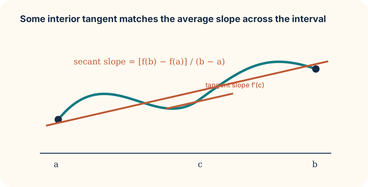
For $f(x)=x^2$ on $[1,3]$, the average slope is

$$\frac{f(3)-f(1)}{3-1}=\frac{9-1}{2}=4.$$

Since $f'(x)=2x$, solve $2c=4$ to obtain $c=2$. The polynomial meets both hypotheses, and two lies in $(1,3)$, so the result verifies the theorem in this case. The calculation comes after, not instead of, checking continuity and differentiability.

Hypotheses prevent false conclusions

A function with a jump can have an average endpoint slope without tracing the intermediate behavior needed for a matching tangent. A function with a corner, such as $|x|$ on $[-1,1]$, is continuous but not differentiable at the interior point zero. Its endpoint average slope is zero, yet no differentiable interior point has derivative zero: the slopes are $-1$ on the left and $1$ on the right. This example shows why both hypotheses are necessary.

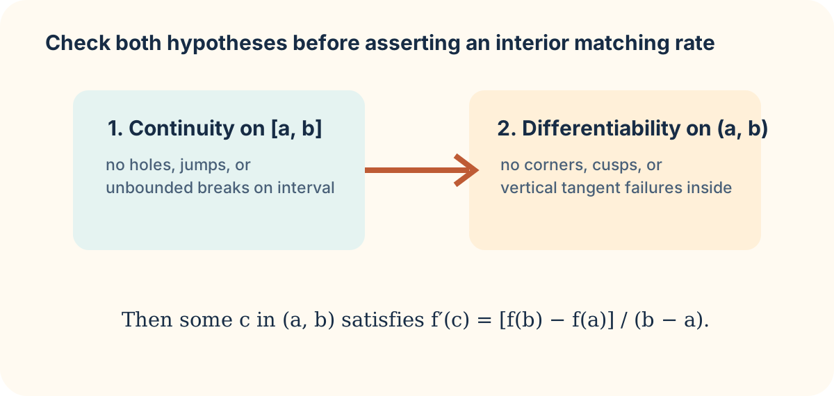
Endpoints matter differently for the two conditions. Continuity is required at the endpoints because the secant uses endpoint values. Differentiability is required only in the interior because there is no two-sided tangent calculation within the interval at an endpoint. Read bracket notation carefully: $[a,b]$ includes endpoints, while $(a,b)$ excludes them.

Rolle’s Theorem is the special case of MVT where $f(a)=f(b)$. The average slope is then zero, so some interior point has $f'(c)=0$. This helps explain why a smooth curve that begins and ends at the same height must have a horizontal tangent somewhere between, provided it satisfies the hypotheses.

Derivative signs control whole intervals

If $f'(x)>0$ for every interior input of an interval, MVT proves that $f$ is increasing there. Choose any two inputs $x_1<x_2$. MVT supplies a point $c$ between them where

$$\frac{f(x_2)-f(x_1)}{x_2-x_1}=f'(c)>0.$$

Because the denominator is positive, the numerator must be positive, so $f(x_2)>f(x_1)$. The proof upgrades local positive slopes into a global ordering statement. A parallel argument shows that $f'(x)<0$ implies $f$ is decreasing.

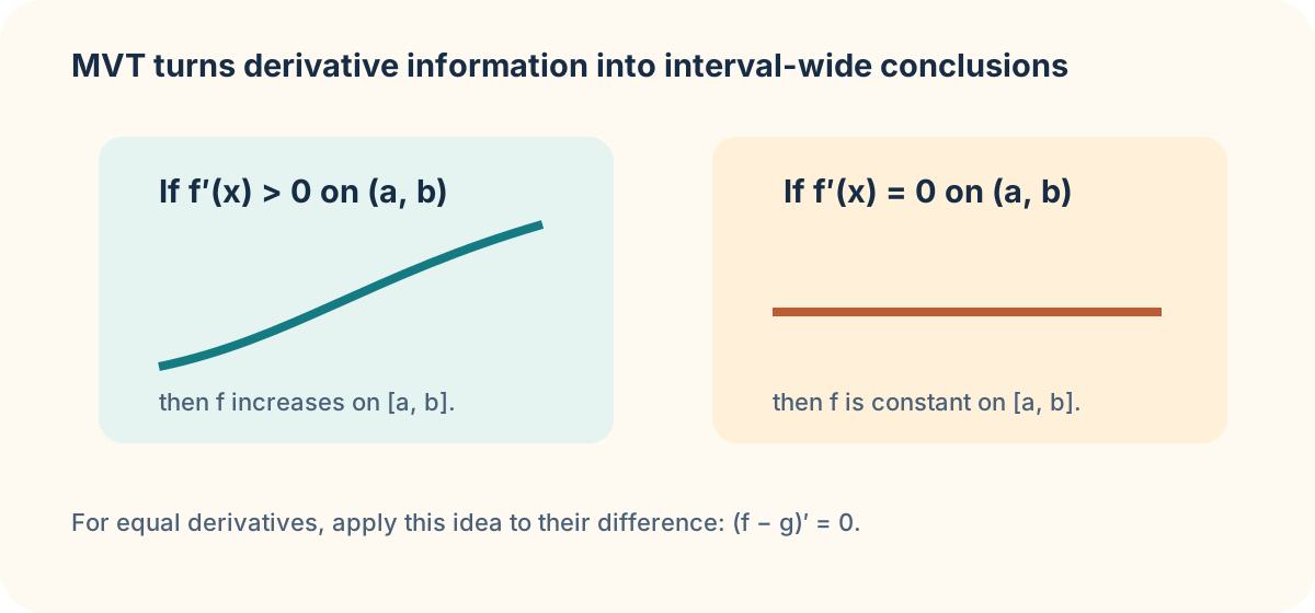
If $f'(x)=0$ throughout an interval, then $f$ is constant there. More generally, if $f'(x)=g'(x)$ throughout an interval, then $(f-g)'(x)=0$, so $f-g$ is constant. This explains why two antiderivatives of the same function differ by a constant, an idea that will return in the integration unit.

These conclusions need interval-wide derivative information. Knowing $f'(2)>0$ tells us only a local fact near two. It does not prove the function increases over every possible input. Name the interval on which the sign condition holds before making a monotonicity claim.

A rate interpretation with units

If $s(t)$ is position in meters over time in seconds, then the MVT equation is

$$v(c)=\frac{s(b)-s(a)}{b-a}.$$

Both sides have units $\frac{\mathrm{m}}{\mathrm{s}}$. If a runner covers $400\,\mathrm{m}$ in $80\,\mathrm{s}$ and the position function is continuous and differentiable during the run, then at some time the instantaneous velocity is $5\,\frac{\mathrm{m}}{\mathrm{s}}$. The theorem does not prove that the runner maintains that velocity, only that it occurs at least once.

Practice by applying MVT to $f(x)=x^3-x$ on $[-1,2]$. Check the hypotheses, compute the average slope, solve for all possible $c$ values, and confirm they lie inside the interval. Then explain why the conclusion says “at least one.” This theorem supplies a rigorous language for moving between local derivatives and global behavior, which is exactly what graph analysis needs next.