Limit Laws and Direct Substitution

Once a two-sided limit is known to exist, algebra can often compute it efficiently. Limit laws say that sums, products, quotients, powers, and suitable compositions preserve limiting destinations. Direct substitution is the familiar practical result for expressions continuous at the target. It is powerful precisely because it rests on structure, not because a limit symbol means “plug in.” This lesson makes that distinction explicit.

We will state the core laws, use them on polynomial and rational models, and diagnose the cases in which substitution produces an indeterminate form. We will also track denominator restrictions and composite-function domains. The guiding question is: when does evaluating an expression at the target faithfully report nearby behavior? The next lesson handles the nontrivial cases where the shortcut stops working.

By the end, you should apply limit laws with their hypotheses, compute continuous polynomial and rational limits, and explain why a nonzero denominator matters. You should recognize that substitution yielding $\frac00$ is not an answer. You should also use a limit calculation to justify a continuity claim. Efficient computation should preserve the conceptual evidence established in earlier lessons.

Limit laws transfer known destinations

Suppose $\lim_{x\to a}f(x)=L$ and $\lim_{x\to a}g(x)=M$. The sum, difference, product, and constant-multiple laws state

$$\lim_{x\to a}[f(x)\pm g(x)]=L\pm M, \qquad \lim_{x\to a}[f(x)g(x)]=LM,$$

and $\lim_{x\to a}[cf(x)]=cL$ for a constant $c$. Each conclusion inherits nearby control from the two component functions.

The quotient law requires one additional condition:

$$\lim_{x\to a}\frac{f(x)}{g(x)}=\frac{L}{M}, \qquad M\ne0.$$

The nonzero condition prevents a denominator from approaching zero, where division can become unbounded or indeterminate. Writing the condition is part of using the law correctly.

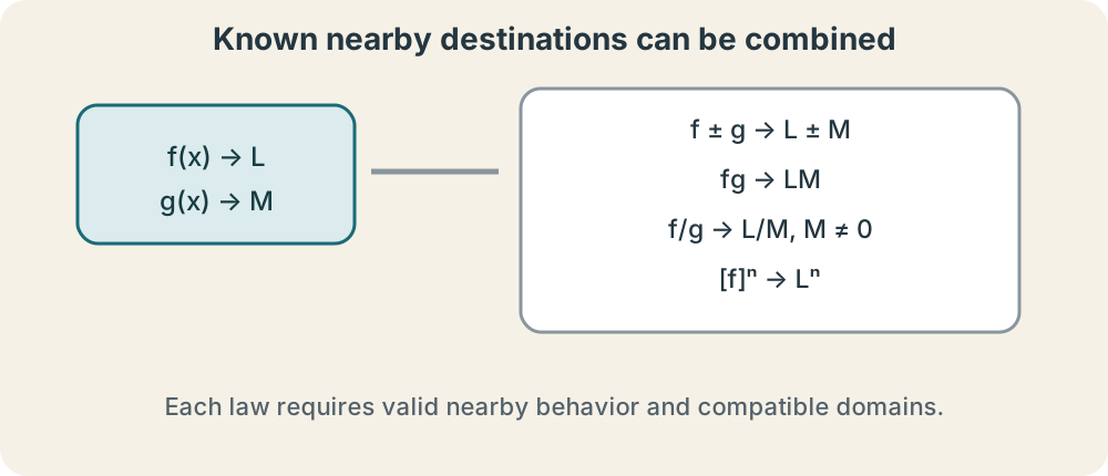
Powers and roots are also governed by continuity on their appropriate domains. If $f(x)$ approaches $L$, then $[f(x)]^n$ approaches $L^n$ for a positive integer $n$. An even root requires the relevant nearby outputs to remain nonnegative in the real setting. Laws do not erase domains. They state how valid nearby behavior is preserved under permitted operations.

Polynomials are continuous everywhere

A polynomial is built from constants and the identity function using addition, multiplication, and nonnegative integer powers. The limit laws therefore show that every polynomial is continuous for every real input. For

$$p(x)=3x^3-2x^2+5x-7,$$

we may compute $\lim_{x\to2}p(x)$ by evaluating $p(2)=15$. This is direct substitution justified by continuity.

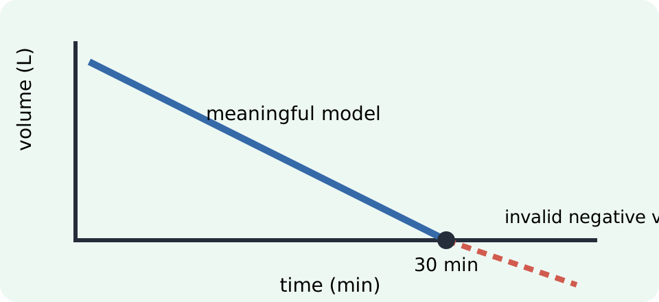
Keep the calculation legible by naming the target and carrying units when a model requires them. If $p(t)$ measures height in meters and $t$ measures seconds, then $p(2\,\mathrm{s})$ should be reported in meters. Coefficients must carry compatible units for the terms to be added. Limit laws preserve dimensions as well as numerical operations.

Substitution is a conclusion after the function class has been recognized. It is not necessary to construct a table every time a polynomial appears. Earlier evidence has established what a limit means; the laws now provide a theorem-backed shortcut. A reader should be able to state the reason: polynomials are continuous at the target.

Rational functions require a denominator check

A rational function is a quotient of polynomials. It is continuous wherever its denominator is nonzero. For

$$r(x)=\frac{x^2+3x-1}{x-4},$$

the denominator at $x=2$ is $-2$, so direct substitution is justified. The limit is $\frac{9}{-2}=-\frac92$. The horizontal fraction bar preserves the quotient’s structure and makes the nonzero denominator condition visible.

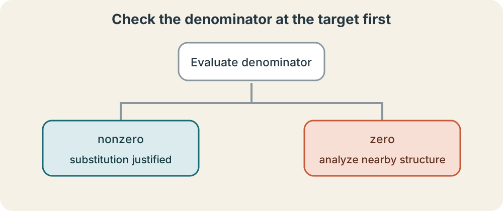
At $x=4$, direct substitution produces a zero denominator. The quotient law cannot be applied. The failure may represent a vertical asymptote, a removable hole, or another behavior depending on the numerator and nearby structure. The correct response is not “the limit is undefined” without further analysis. It is to move to the next lesson’s restructuring tools.

Rational models also have contextual domains. A formula may be algebraically defined at a time value that lies outside the experiment’s stated interval. Continuity within an expression does not authorize extrapolation. First check mathematical domain, then contextual domain, then use the appropriate law. A computationally valid number can still be an invalid model prediction.

Composition requires compatible nearby behavior

If $\lim_{x\to a}g(x)=M$ and an outer function $f$ is continuous at $M$, then

$$\lim_{x\to a}f(g(x))=f(M).$$

This composition law explains direct substitution in expressions such as $\sqrt{3x+1}$ at $x=1$. The inside approaches four, and square root is continuous at four, so the complete expression approaches two. The inner and outer domains must both be checked.

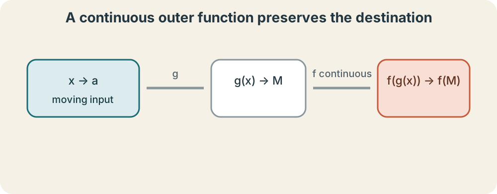
For $\ln(3x-2)$ at $x=1$, the inner expression approaches one, which lies in the positive real domain of logarithm. Direct substitution gives zero. At $x=\frac23$, however, the inner expression approaches zero and the real logarithm is not continuous there because it is not defined. A formula’s outer operation can determine whether the shortcut applies.

Trigonometric functions are continuous for all real inputs when angles are measured in radians. Thus $\lim_{x\to0}\sin(5x)=0$ follows by composition. Radian measure matters because it preserves the standard calculus scaling of trigonometric limits and derivatives. Units inside trig inputs must still be dimensionless or converted consistently.

Diagnose before you calculate

A useful workflow begins with a domain check. Next, substitute as a diagnostic. If the result is an ordinary real value and the expression is continuous at the target, state the continuity justification and report the limit. If the result is $\frac00$, a zero denominator, an invalid root, or an invalid logarithm, stop treating substitution as an answer. Classify the obstruction and choose an appropriate next method.

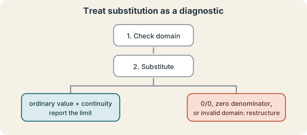
Avoid two common errors. Do not cancel expressions before recording the original restrictions. Do not declare every $\frac00$ limit nonexistent. The same indeterminate form can conceal a removable factor, a radical difference, or a more complicated structure. Algebra must respond to the form and to the nearby domain.

The laws also do not prove a limit exists when a component limit fails. A quotient with a jump in its numerator inherits that difficulty. Check directional existence first when the representation suggests a discontinuity. Laws are tools for combining established local behavior. They are not a substitute for the existence analysis in the preceding lessons.

Synthesis and transition

Compute $\lim_{x\to3}(2x^3-x+4)$, $\lim_{x\to1}\frac{x^2+1}{x+2}$, and $\lim_{x\to0}\sqrt{4+x}$. State the law or continuity fact that justifies each substitution. For every rational expression, evaluate the denominator separately before calculating the quotient. Add units if you choose to interpret one expression as a model.

Then test $\lim_{x\to2}\frac{x^2-4}{x-2}$ by substitution. Explain why the output is not a limit value. Name the algebraic feature that should be investigated next, and predict which restructuring tool may help. Compare this diagnostic result with the rational example whose denominator stayed nonzero. The difference lies in the target’s nearby domain, not in the typography of the fraction alone.

Limit laws make computation efficient when their hypotheses hold. Continuous functions allow direct substitution because their nearby behavior agrees with their assigned values. Rational functions add a denominator condition, and compositions add an outer-domain condition. When those checks fail, the limit question remains open rather than answered incorrectly. The next lesson develops factoring, rationalization, and common-denominator techniques for those nontrivial finite limits.