Graphing with First and Second Derivatives

A graph sketch in calculus is an evidence-based argument. The original function supplies domain, intercepts, and asymptotes. The first derivative supplies increasing and decreasing behavior as well as critical-point candidates. The second derivative supplies concavity and possible inflection points. No single derivative calculation replaces the others, and a reliable sketch records which claim comes from which evidence.

This lesson builds a practical sequence for analyzing a function without relying on a graphing device to decide the mathematics. The goal is not an artistically perfect curve. It is a graph whose important features are justified: where it is defined, where it rises or falls, where it bends, and what behavior occurs near excluded inputs or at infinity. A plotting tool can check a completed analysis, but it should not replace the reasoning.

By the end, you should organize a derivative sign chart, classify extrema with the first or second derivative test, identify genuine inflection points, and combine this information into a coherent sketch. You should state domain restrictions before interpreting a derivative. The next lessons apply the same rate structure to connected quantities and numerical root finding.

Establish the original function’s structure first

Start with the domain. A rational function is undefined where its denominator is zero, and a logarithm requires a positive argument. Then find convenient anchors such as intercepts and values at simple inputs. Analyze vertical or horizontal asymptotes when appropriate. These features constrain every later sketch; no derivative sign can give a function a value where its original formula is undefined.

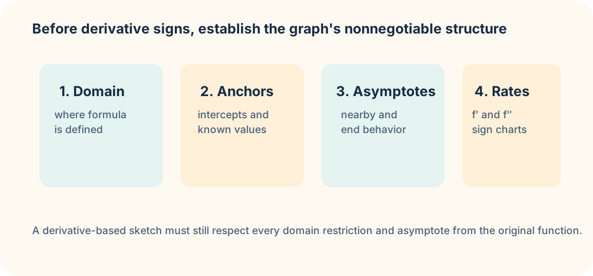
For $f(x)=\frac{x+1}{x-2}$, the domain excludes $x=2$. The vertical asymptote is $x=2$, while polynomial degree comparison gives horizontal asymptote $y=1$. Its derivative may tell where each branch rises or falls, but it cannot erase the discontinuity. Separate the domain into intervals at every point where the function or derivative is undefined before making a sign chart.

End behavior and derivative behavior answer different questions. An asymptote describes what function values approach near a boundary or far away. A positive derivative describes increasing behavior locally across an interval. A function may increase while approaching a horizontal asymptote, or it may decrease toward one. Keep these statements distinct and then combine them in the final sketch.

Use the first derivative to organize rise and fall

Solve $f'(x)=0$ and locate where $f'$ is undefined while $f$ remains defined. These are critical-point candidates. Mark them on a number line along with domain breaks. Choose a test input in each interval and determine the sign of $f'$. Positive sign means increasing; negative sign means decreasing. The Mean Value Theorem supports the interval-wide conclusion when the derivative retains that sign.

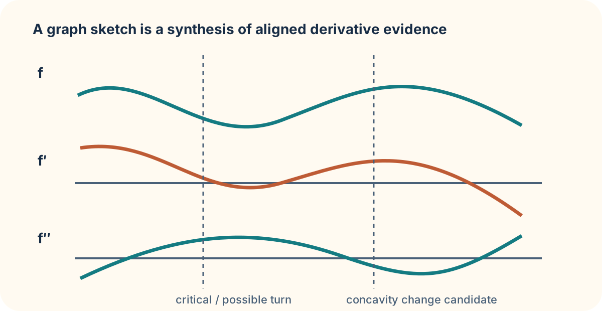
If the sign changes from positive to negative at a critical point, classify a local maximum. If it changes from negative to positive, classify a local minimum. If the sign does not change, do not force an extremum. For example, $f(x)=x^3$ has derivative zero at zero but remains increasing, so zero is not a maximum or minimum. A sign chart is stronger evidence than a zero derivative alone.

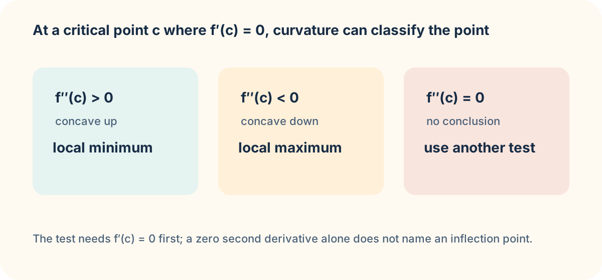
The second derivative test can sometimes shorten the work. At a critical point $c$ with $f'(c)=0$, positive $f''(c)$ indicates concave up and a local minimum; negative $f''(c)$ indicates concave down and a local maximum. If $f''(c)=0$, the test is inconclusive. Return to a first-derivative sign chart or another method.

Use the second derivative to analyze bending

Solve $f''(x)=0$ and locate points where $f''$ is undefined, then test the sign of $f''$ over resulting intervals. Positive means concave up; negative means concave down. An inflection point requires the original function to be defined and concavity to change. A zero second derivative without a sign change is not enough.

For $f(x)=x^3$, $f''(x)=6x$ changes from negative to positive at zero, so the graph has an inflection point at $(0,0)$. For $f(x)=x^4$, $f''(0)=0$ but $f''$ is nonnegative on both sides, so the graph remains concave up and has no inflection point there. The sign change is the criterion, just as it was for the first derivative test.

Concavity explains changes in slopes, not whether function values are positive. A graph below the horizontal axis may be concave up, and a graph above it may be concave down. Describe the bending in terms of tangent slopes increasing or decreasing. This language prevents a common confusion between a graph’s height and its curvature.

Assemble and check the final sketch

Draw a curve that respects every confirmed feature: domain breaks, anchors, asymptotes, intervals of increase/decrease, extrema, and concavity. Do not invent exact coordinates that the algebra did not establish. Use smooth connections only where the function is continuous and differentiable as required. Label important inputs and output values so a reader can trace each graphical claim back to the sign chart or original function.

As practice, analyze $f(x)=x^3-3x$. Find intercepts, critical points, intervals of increase/decrease, and concavity. Then compare your sketch with a graphing tool only after completing the table. If a discrepancy appears, ask which evidence was misread rather than changing the sketch by eye. This method becomes especially valuable in the next lesson, where relationships among changing quantities are translated into derivatives.