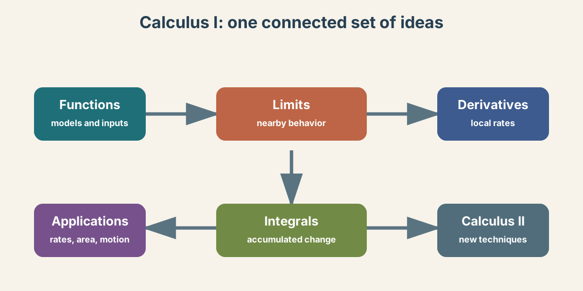
Calculus I Synthesis and Calculus II Readiness

Calculus I is not a list of independent tricks. It is a language for describing quantities that depend on one another and for making careful claims about change. A function gives the model, a limit asks what happens nearby, a derivative records a local rate, and an integral accumulates many small contributions. The point of this final lesson is to make that architecture visible so that later methods have a place to attach.

You have also learned that calculation is only part of a mathematical answer. A derivative can be found correctly and then interpreted with the wrong units. A definite integral can be evaluated correctly and then called distance when it actually represents signed displacement. Every complete solution identifies the quantity, states what the independent variable means, and checks whether the result is plausible in context.

This synthesis is a beginning rather than a finish line. Calculus II will ask you to integrate more complicated functions, study infinite processes, and extend familiar ideas into new settings. Those topics are manageable when the ideas below remain connected to their meanings.

The central network: function, limit, derivative, integral

Start with a function such as $s(t)$, where $s$ is position in meters and $t$ is time in seconds. The notation is compact, but every symbol has a job: $s$ names the output quantity, $t$ names the input, and $s(t)$ is the position associated with a particular time. A graph, a table, a formula, and a verbal description can all represent the same relationship. Moving among those representations is not decoration; it is how you test whether a model is being interpreted correctly.

A limit focuses on behavior near an input. The expression $\lim_{t\to a}s(t)=L$ says that outputs of $s(t)$ can be made close to $L$ by choosing times sufficiently close to $a$, without requiring $t=a$. That nearby viewpoint explains why the derivative can be defined even though its difference quotient divides by a time difference that becomes arbitrarily small. Continuity supplies a reliable bridge between nearby behavior and a function’s actual value when its conditions are met.

The derivative $s'(t)$ is the instantaneous rate of change of position with respect to time, so its units are $\frac{\mathrm{m}}{\mathrm{s}}$. The definite integral $\int_a^b s'(t)\,dt$ accumulates that rate and has units of meters. The Fundamental Theorem of Calculus connects these two operations: under appropriate conditions, accumulated rate recovers net change. This is why a coherent Calculus I course moves from functions and limits to rates and then to accumulation.

A dependable workflow for unfamiliar problems

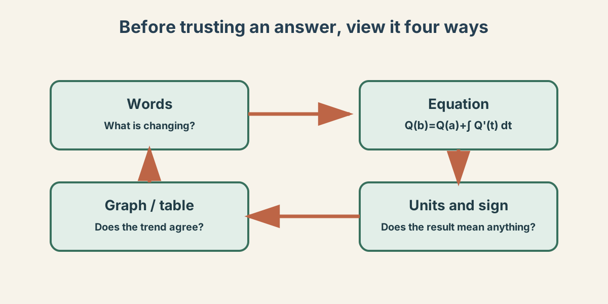
When a problem looks unfamiliar, begin before choosing a rule. Identify the independent variable, its units, the dependent quantity, and whether the question asks about a value, a local rate, or an accumulated change. For example, if $R(t)$ has units $\frac{\mathrm{L}}{\mathrm{min}}$, then $\int_0^{10}R(t)\,dt$ has units of liters. This unit check predicts the kind of answer before any antiderivative is found.

Next, make a representation check. Read the words, inspect any graph or table, write an equation, and follow the signs. A negative derivative means the modeled output is decreasing with the chosen input; it does not mean that the output itself is negative. A negative velocity contributes negatively to displacement, while its absolute value contributes positively to distance. These distinctions prevent many errors that symbolic fluency alone cannot catch.

Finally, compute with a named reason for each step and return to the context. If you use the Chain Rule, name the inner and outer functions. If you use a definite integral, say what each region contributes and whether cancellation is appropriate. Report units with the final value, round only when the measurement context supports it, and write one sentence interpreting the result. That final sentence is evidence that the calculation answered the question asked.

What deserves continued practice

The most transferable Calculus I skill is recognizing structure. Product, quotient, and chain rules are not random operations: each describes how a composite quantity changes. The same is true of integration methods. Substitution reverses a recognizable chain-rule pattern, and the Fundamental Theorem evaluates accumulated change by linking it to an antiderivative. Practice should therefore include deciding why a method fits, not merely carrying it out.

Keep revisiting functions and algebra. Factoring, solving equations, simplifying rational expressions, working with exponents and logarithms, and reading graphs are prerequisites that reappear whenever calculus methods become technical. A stalled calculus problem is often an algebra or representation problem in disguise. Repairing that foundation is efficient, because it improves every later topic instead of only one exercise type.

Use errors as diagnostic information. If an answer has impossible units, revisit the differential and the variable. If a graph suggests a maximum but the derivative test says otherwise, locate the sign or domain mistake. If a numerical estimate and an exact answer disagree sharply, check interval width, scale, and whether a signed quantity was mistaken for a total. A habit of checking gives you a way to recover rather than a reason to guess.

Crossing the bridge to Calculus II

Calculus II extends integration beyond the cases handled comfortably by substitution and elementary antiderivatives. You will learn additional techniques because different function structures require different reversals of differentiation. You will also study improper integrals and infinite series, where a limit controls a process that does not stop after finitely many steps. The same language of approximation, convergence, and justified conclusions begins in the limit work you have already completed.

The transition is smoother when you can explain the ideas of Calculus I out loud. You should be able to say why $\frac{d}{dx}\int_a^x f(t)\,dt=f(x)$ under the theorem’s hypotheses, why a derivative’s units are output units divided by input units, and why an integral of a rate returns the original quantity’s units. You should also recognize that a formula is a claim with assumptions: domain restrictions, continuity conditions, and a meaningful model all matter.

Keep the course synthesis narrative nearby as a final self-check. It asks you to model a realistic setting before revealing a solution path, which is precisely the kind of judgment later courses require. If you can translate between its story, graph, formulas, and units, you are ready to meet new tools without losing the meaning that makes them useful.

Course close: a compact readiness check

Choose a quantity from a familiar setting, such as water in a tank, a vehicle’s position, or money in an account. Define a function for the quantity and state its units. Then define a rate function, explain the derivative’s units, and write the definite-integral expression for net change over a stated interval. Do not calculate yet; the goal is to make the model legible before computation begins.

Now ask two interpretation questions. Could the rate be negative, and what would that mean? Does the context require signed net change, or a total that needs absolute values or separate positive and negative components? These questions force a distinction that appears throughout physics, economics, and data analysis. They also make clear why calculus is a reasoning discipline rather than a contest of formula recall.

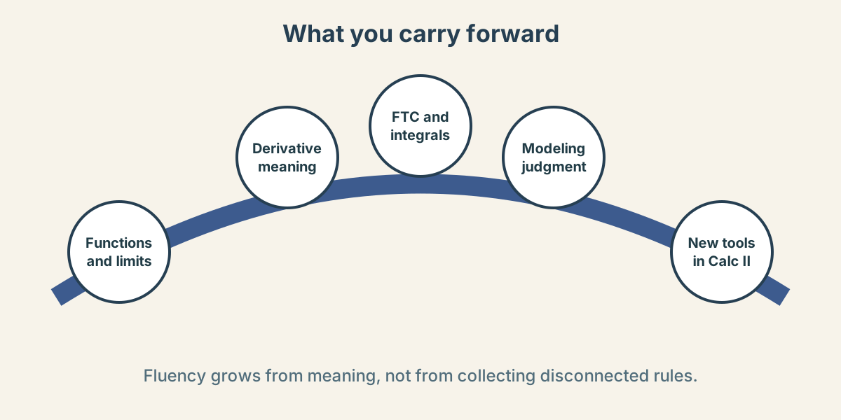
If you can construct and explain this model, you have the core preparation for the next course. Keep practicing short, complete solutions: identify the quantity, select a justified method, calculate accurately, and interpret the result with units. That sequence is the durable result of Calculus I.