Average Rate of Change and Secant Slope

A function compares outputs across inputs, but a rate compares how much the output changes with how much the input changes. That extra division makes interval length visible. A temperature rise of $10\,{}^\circ\mathrm{C}$ in $2\,\mathrm{min}$ and the same rise in $20\,\mathrm{min}$ represent different rates. Average rate of change captures this distinction. Geometrically, the same quotient is the slope of a secant line through two graph points.

This lesson develops one idea through context, tables, graphs, and formulas. We will preserve the order of endpoints, attach compound units, and interpret the sign of a rate. We will also examine why nonlinear functions have interval-dependent average rates. The guiding question is: what does one quotient say about change across an entire interval? The next lesson will turn the fixed interval into a movable symbolic interval.

By the end, you should compute and interpret $\frac{f(b)-f(a)}{b-a}$, identify its units, and connect it to secant slope. You should distinguish total change from rate of change. You should explain why reversing both endpoints does not change the quotient. You should compare rates across intervals of unequal length. You should also recognize that an average rate does not automatically describe every moment inside the interval.

Change requires two ordered endpoints

Let an input move from $a$ to $b$. The input change is $\Delta x=b-a$, and the corresponding output change is $\Delta f=f(b)-f(a)$. The triangular symbol $\Delta$ is read “change in”; it is not a variable multiplied by $x$. Both differences must use the same endpoint order. Mixing $f(b)-f(a)$ with $a-b$ reverses the sign without a mathematical reason.

The average rate of change of $f$ on $[a,b]$ is

$$\frac{\Delta f}{\Delta x}=\frac{f(b)-f(a)}{b-a},\qquad a\ne b.$$

The denominator must be nonzero because an interval needs two distinct inputs. The numerator measures net output change, not the total variation accumulated along a complicated path. Dividing by the input change normalizes the comparison to one input unit. This makes rates from intervals of different lengths comparable.

Suppose a vehicle’s position changes from $40\,\mathrm{m}$ at $2\,\mathrm{s}$ to $136\,\mathrm{m}$ at $8\,\mathrm{s}$. The position change is $96\,\mathrm{m}$ and the time change is $6\,\mathrm{s}$. Its average velocity is $\frac{96\,\mathrm{m}}{6\,\mathrm{s}}=16\,\frac{\mathrm{m}}{\mathrm{s}}$. The unit is a fraction because the quantity is meters per second. A bare answer of $16$ omits the physical meaning.

Tables organize rate evidence

A useful table keeps inputs, outputs, changes, and rates in separate columns. The input and output headings contain their original units. The change columns inherit those units. The rate column uses output units divided by input units. This layout makes dimensional mistakes and reversed subtractions easier to detect.

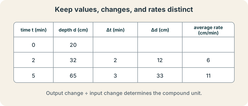
Consider water depth measurements of $20\,\mathrm{cm}$ at $0\,\mathrm{min}$, $32\,\mathrm{cm}$ at $2\,\mathrm{min}$, and $65\,\mathrm{cm}$ at $5\,\mathrm{min}$. From zero to two minutes, the average rate is $6\,\frac{\mathrm{cm}}{\mathrm{min}}$. From two to five minutes, it is $11\,\frac{\mathrm{cm}}{\mathrm{min}}$. The larger second rate signals faster average increase during that interval. It does not prove the depth increased at a constant $11\,\frac{\mathrm{cm}}{\mathrm{min}}$ at every moment.

A table contains finite interval evidence. Sampling more often can reveal changing patterns, but it does not create instantaneous information by itself. Measurement uncertainty also propagates into differences, especially when two close readings are subtracted. A small denominator can magnify noise in the quotient. These limitations become important when intervals shrink in the limits unit.

Secant slope is the same quotient

The graph points associated with inputs $a$ and $b$ are $(a,f(a))$ and $(b,f(b))$. The line through these two points is a secant line. Its slope is rise divided by run, which is exactly $\frac{f(b)-f(a)}{b-a}$. Average rate and secant slope are therefore two interpretations of one calculation. Context supplies the units while geometry supplies the line.

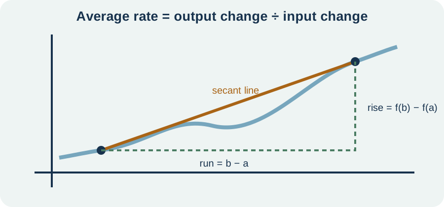
On a position-versus-time graph, secant slope is average velocity. On a temperature-versus-time graph, it is average temperature change per unit time. On a cost-versus-quantity graph, it is average additional cost per added item. The axes determine the rate’s meaning. A visually identical slope number can represent different physical quantities when the axis units differ.

The sign of the secant slope reports net directional behavior. Positive slope means the later output is larger when $b>a$. Negative slope means it is smaller. Zero slope means the endpoint outputs agree, even if the function varied between them. An average rate can therefore be zero across an interval that contains substantial rise and fall.

Interval choice matters for nonlinear functions

For a linear function $f(x)=mx+c$, every average rate equals $m$. Substitution gives

$$\frac{m b+c-(m a+c)}{b-a}=\frac{m(b-a)}{b-a}=m.$$

The constant-rate property characterizes the linear family. Every secant line lies on the same graph. Interval location and length do not change the rate.

For $f(x)=x^2$, the average rate on $[a,b]$ is

$$\frac{b^2-a^2}{b-a}=\frac{(b-a)(b+a)}{b-a}=a+b.$$

The result depends on both endpoints. On $[0,2]$ the rate is $2$, while on $[2,4]$ it is $6$. Both intervals have length two, yet the second lies where the parabola is steeper. Equal interval lengths do not imply equal rates for nonlinear functions.

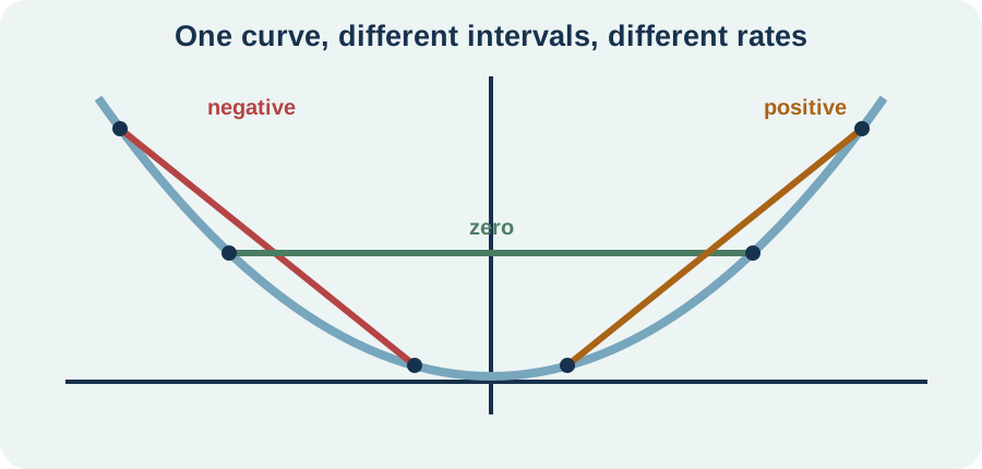
Changing interval length while fixing one endpoint also changes the result. For $x^2$ from $x=1$ to $x=1.5$, the rate is $2.5$. From $x=1$ to $x=1.1$, it is $2.1$. The secant lines rotate as the second endpoint moves. This observation motivates the later question of whether the slopes approach a stable local value.

Synthesis and transition

For $T(t)=18+3t-0.2t^2$, where $T$ is degrees Celsius and $t$ is minutes, compute the average rate on $[0,5]$ and $[5,10]$. Show both endpoint differences and attach $\frac{{}^\circ\mathrm{C}}{\mathrm{min}}$ to each result. Interpret the sign and compare the intervals. Sketch the associated secant lines without claiming they show instantaneous rates.

Then design a function whose average rate on $[0,4]$ is zero even though it is not constant there. Provide a formula or labeled graph and explain why the endpoint quotient misses internal variation. Reverse the endpoint order and confirm that the quotient remains unchanged because both numerator and denominator reverse sign. State what would go wrong if only one difference were reversed. Use complete sentences rather than a list of arithmetic steps.

Average rate of change measures net output change per input change across a nonzero interval. The secant slope is its geometric form, and its compound units come from the graph axes or modeled quantities. Linear functions keep the same rate on every interval, while nonlinear functions generally do not. The next lesson introduces movable difference quotients that encode a family of secant intervals symbolically. That notation will prepare the transition from average change to local change.