Directional Agreement and Two-Sided Existence

An ordinary limit makes one claim about every locally available approach direction. Separate one-sided limits reveal whether that claim is possible. If the left and right destinations exist and match, they combine into one two-sided limit. If they differ or one side fails to stabilize, no finite number can describe the complete approach. Directional agreement is therefore the existence criterion, not merely a checking trick.

This lesson derives the criterion, applies it to piecewise functions and jumps, and distinguishes finite disagreement from unbounded behavior. We will also revisit endpoints so the theorem is not applied outside its domain assumptions. A real-world switching example will connect the symbols to model behavior. The guiding question is: when can two directional statements be compressed into one? The next lesson will compute limits efficiently once existence is conceptually secure.

By the end, you should state and justify the two-sided existence theorem, apply it to graphs and formulas, and explain nonexistence by naming the conflict. You should never average unequal one-sided limits. You should distinguish a finite limit from infinite notation. You should use domain-aware endpoint conventions. You should also communicate the difference between discontinuity caused by a jump and a removable point mismatch.

Derive the existence criterion

Suppose $\lim_{x\to a^-}f(x)=L$ and $\lim_{x\to a^+}f(x)=L$. Every sufficiently nearby allowed input other than $a$ lies either to the left or right. The first statement controls outputs on the left, and the second controls outputs on the right. Because both use the same destination, all nearby outputs can be made close to $L$. Therefore the ordinary limit exists and equals $L$.

Conversely, if $\lim_{x\to a}f(x)=L$, the claim already controls every sufficiently nearby allowed input. Restricting those inputs to the left cannot destroy the guarantee. Restricting them to the right cannot destroy it either. Both one-sided limits must therefore equal $L$. The logic works in both directions.

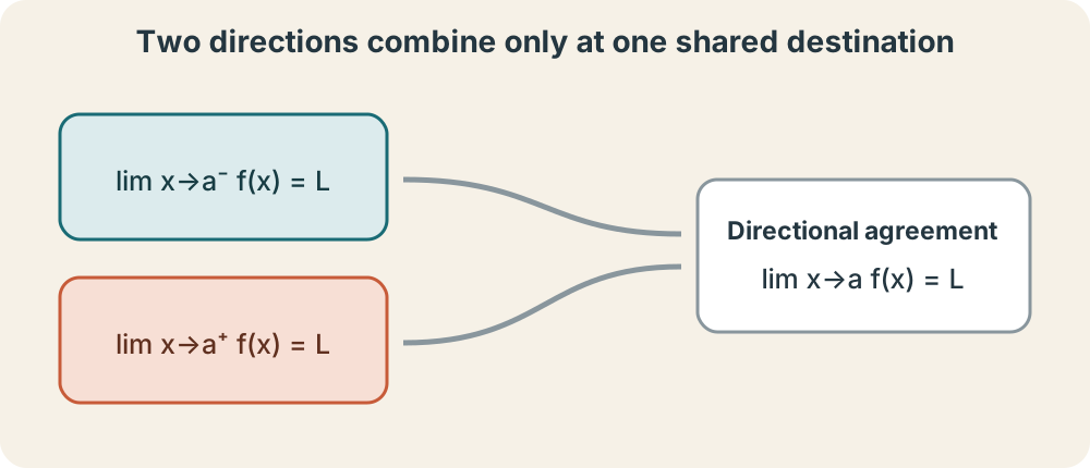
The theorem is written

$$\lim_{x\to a}f(x)=L \quad\Longleftrightarrow\quad \lim_{x\to a^-}f(x)=L \text{ and } \lim_{x\to a^+}f(x)=L.$$

The double arrow means each side implies the other. The repeated $L$ is essential. Merely having two one-sided limits is not enough.

A jump defeats the common destination

For a step-like function, suppose the left-hand limit at $a$ is one and the right-hand limit is three. Each directional limit exists as a finite value. Because $1\ne3$, no single number describes both approaches. The ordinary two-sided limit does not exist. The reason should be stated explicitly: the one-sided limits disagree.

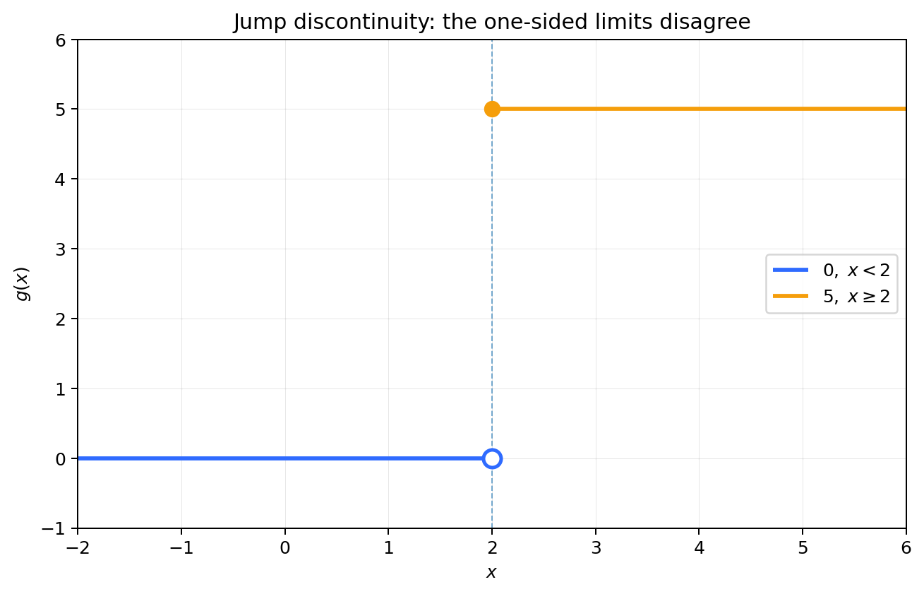
Averaging the values to obtain two has no mathematical basis. Neither branch approaches two. Choosing the filled point value is equally irrelevant because one isolated output cannot repair surrounding disagreement. The function can be defined at the target and still lack a limit there. Limit existence belongs to the neighborhood.

A jump is different from a removable discontinuity. At a removable mismatch, both branches approach the same $L$ while $f(a)$ is missing or different. The limit exists and the point can be repaired. At a jump, no reassignment of the single point can make the directional destinations agree. The distinction determines whether continuity can be restored locally by changing one value.

Piecewise parameters enforce agreement

Consider

$$p(x)= \begin{cases} kx+1, & x<2,\\ x^2+k, & x\ge2. \end{cases}$$

The left-hand destination is $2k+1$, and the right-hand destination is $4+k$. A two-sided limit exists exactly when $2k+1=4+k$. Solving gives $k=3$, and the common limiting value is seven.

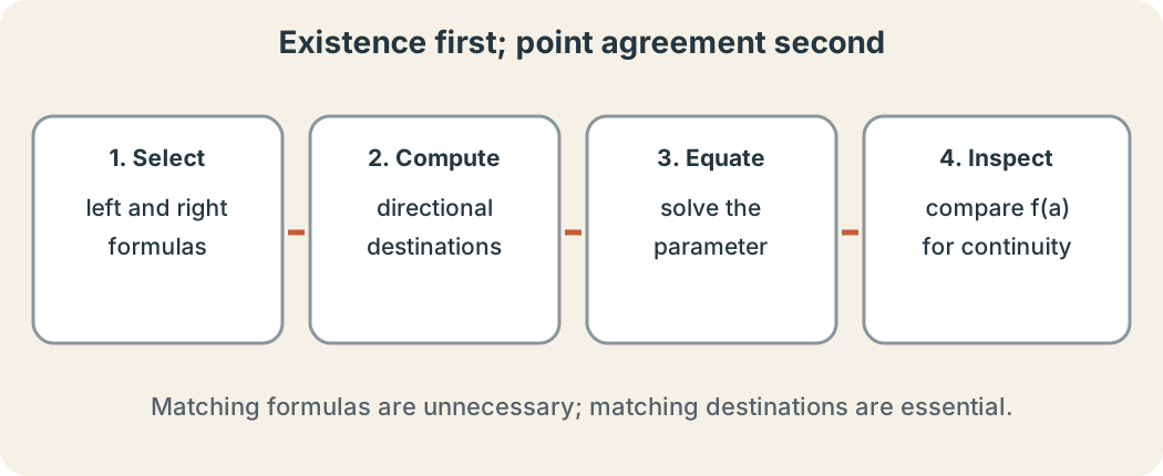
The value at $x=2$ comes from the second branch because it contains equality. For $k=3$, that value is seven, so the function is also continuous. If a separate rule assigned $p(2)=100$, the limit would remain seven but continuity would fail. Existence and point agreement are consecutive questions. Solving both at once without naming them hides the logic.

Parameter problems should follow a stable sequence. Select the left and right branches, compute their nearby destinations, set those destinations equal, solve the resulting equation, and only then inspect the point value if continuity is asked. This routine prevents inequality symbols from being mistaken for endpoint instructions. It also shows why one parameter can remove a jump. The algebra implements the theorem.

Unbounded directional behavior needs different notation

For $r(x)=\frac1x$ at zero, positive inputs produce arbitrarily large positive outputs and negative inputs produce arbitrarily large negative outputs. We write

$$\lim_{x\to0^+}\frac1x=+\infty, \qquad \lim_{x\to0^-}\frac1x=-\infty.$$

These statements describe directional unbounded behavior. Infinity is not a real function value reached at the target.

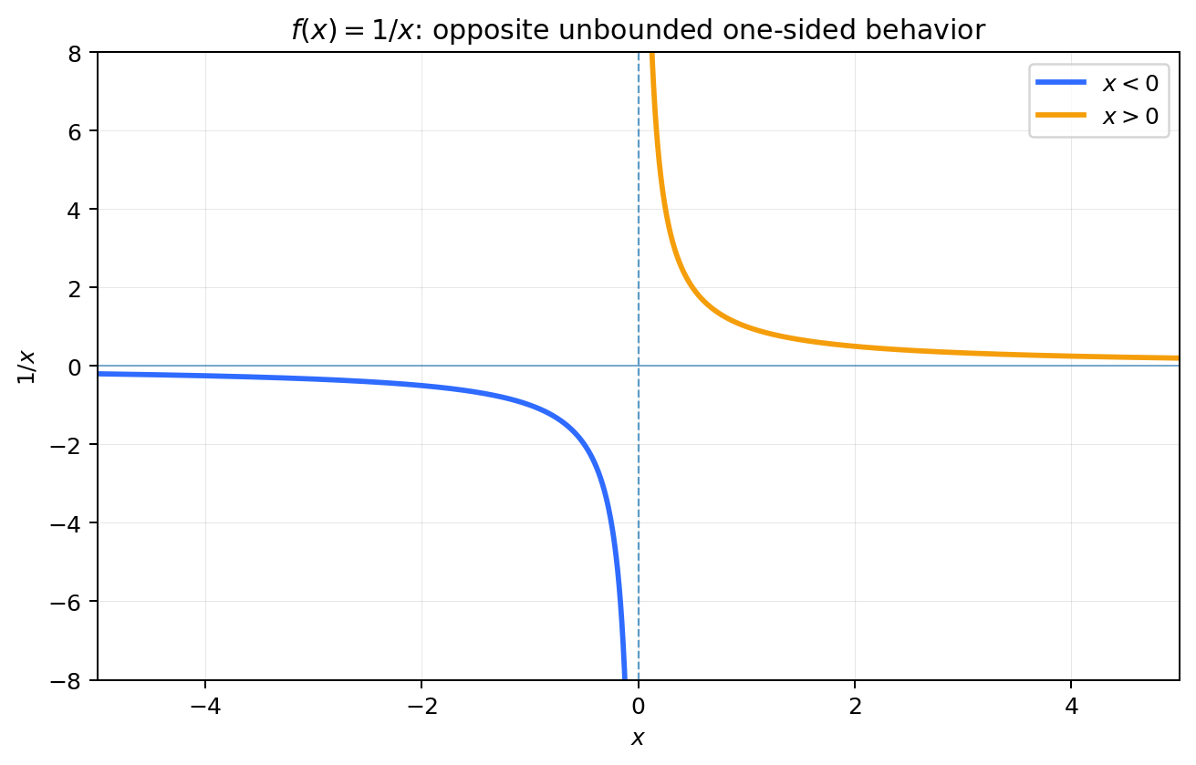
Because the directions have opposite extended behavior, there is no shared two-sided statement of one sign. Even when both sides grow toward $+\infty$, the ordinary finite real limit still does not exist. Some conventions write the two-sided limit as $+\infty$ in the extended sense. The wording must distinguish unbounded growth from convergence to a real number. The theorem for a finite $L$ should not be applied carelessly to infinity.

Oscillation can defeat a one-sided limit before agreement is even considered. The function $\sin(1/x)$ fails to settle as $x\to0^+$ and also as $x\to0^-$. Restricting direction removes left-right mixing but does not guarantee stability within the chosen side. Both existence and agreement matter. The workflow must test each directional claim rather than assume it.

Endpoint conventions and domains

At an interior point with domain values on both sides, the theorem requires both directional limits. At a domain endpoint, only one direction may be locally available. Continuity on a closed interval uses the appropriate one-sided limit at each endpoint. This convention reflects the actual domain. It does not claim that an unavailable direction somehow agrees.

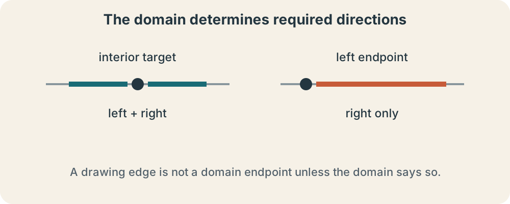
For $f(x)=\sqrt{x}$ on $[0,\infty)$, right-hand behavior at zero determines the endpoint limit. For a function on $(-\infty,5]$, a left-hand limit is relevant at five. In a time model beginning at zero seconds, a right-hand rate may describe startup behavior. Stating the domain makes the convention transparent. Without it, “endpoint” is only a feature of the drawing window.

Do not report that an endpoint two-sided limit “fails because the other side is missing” when the course definition explicitly uses relative-domain approach. Instead, state the available directional limit and the convention being applied. If a problem requests an ordinary real-line two-sided limit, note that the expression lacks domain inputs on one side. Mathematical communication should reveal the convention. Context determines which statement is useful.

A switching-model interpretation

A thermostat changes its command at $T=20\,{}^\circ\mathrm{C}$. Suppose commands approach $40\%$ heater power from below the threshold and $0\%$ from above. The directional limits represent behavior just before and after switching. Their disagreement describes a deliberate jump. A single two-sided limiting command does not exist, regardless of the exact command assigned at the threshold.

If engineers revise the branches so both approach $20\%$, the formulas may remain different while their destinations agree. The two-sided limit is then $20\%$. Assigning exactly $20\%$ at the threshold makes the command function continuous; assigning $35\%$ preserves the limit but creates a removable mismatch. Formula equality is unnecessary. Directional value agreement is decisive.

Units remain attached to the interpretation. Input differences are measured in degrees Celsius, and command outputs in percent of available power. The minus and plus superscripts identify temperatures below and above the threshold, not negative and positive temperatures. The theorem compresses two operational regimes only when they predict the same nearby command. This is a substantive modeling condition.

Synthesis and transition

For the parameterized piecewise function above, verify the value $k=3$ with directional tables and a graph sketch. Then redefine only the point value to be negative five. State the left-hand limit, right-hand limit, ordinary limit, and point value. Explain which property changes and which remain. Use the theorem explicitly in your justification.

Next classify three cases: unequal finite directional limits, opposite unbounded directional behavior, and a domain endpoint with one available side. Write appropriate notation for each and explain why the same phrase “the limit does not exist” would hide important differences. Create one case where the ordinary finite limit exists even though the point value is missing. Compare all four situations in a table.

A two-sided finite limit exists exactly when the required one-sided limits exist and share one real destination. Jumps fail through disagreement, oscillation can fail within a direction, and unbounded behavior requires extended notation. Domain endpoints modify which directions are available. With existence now conceptually secure, the next lesson develops limit laws and direct substitution as efficient computational tools. Computation should follow, not replace, the existence question.