Evidence and Failure in Finite Limits

Understanding a limit statement does not automatically tell us whether it is true. A graph can suggest a destination, a table can quantify approach, and algebra can reveal exact nearby equivalence. Each representation has strengths and limitations. A rigorous reader calibrates the conclusion to the evidence. This lesson develops that discipline and previews three ways a finite limit can fail.

We will estimate limits from graphs and tables, use algebra to justify removable behavior, and compare finite evidence with proof. We will also examine jumps, unbounded behavior, and oscillation. Counterexamples will test tempting universal claims. The guiding question is: what kind of evidence supports a finite limit, and what behavior defeats one? Directional notation will be introduced in the next lesson to formalize left-right agreement.

By the end, you should estimate a finite limit without confusing it with a point value, create a properly organized two-sided table, and state the limits of numerical evidence. You should distinguish jump, unbounded, and oscillatory failure. You should use counterexamples to disprove false claims. You should also select a representation appropriate to the desired conclusion. The goal is honest mathematical inference rather than confident-looking guesswork.

Graphs provide spatial evidence

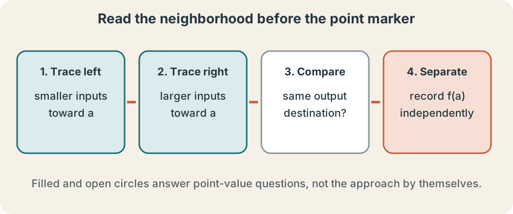
To estimate $\lim_{x\to a}f(x)$ from a graph, trace the curve toward $x=a$ from smaller and larger input values. Watch the output height approached by each branch. Ignore the filled point initially because it represents $f(a)$, not nearby behavior. If both traces approach one height, the graph supports that finite limit. If they approach different heights, no common two-sided destination is visible.

Graph scale matters. A rough plot may hide a small hole, narrow spike, or rapid oscillation. An apparent destination should be reported with precision appropriate to the axes. If the graph is a schematic, exact values require labels or known construction. Saying “the graph suggests a limit near four” is more accurate than inventing many decimal places.

Graphing technology samples and connects points according to its own algorithms. It can miss excluded values or draw through asymptotes. Zooming supplies more visual evidence but does not by itself prove a universal nearby claim. A graph is strongest for structure and weakest for invisible scale-dependent exceptions. Coordinate it with formulas or theorems when exactness matters.

Tables provide numerical evidence

A two-sided table places inputs less than $a$ in one group and inputs greater than $a$ in another. Each group should move progressively closer to the target. Outputs should be recorded with enough precision to reveal stabilization but not fabricated precision beyond the data source. The target row may be omitted because the limit does not require it. Direction labels prevent one-sided sampling from masquerading as a two-sided analysis.

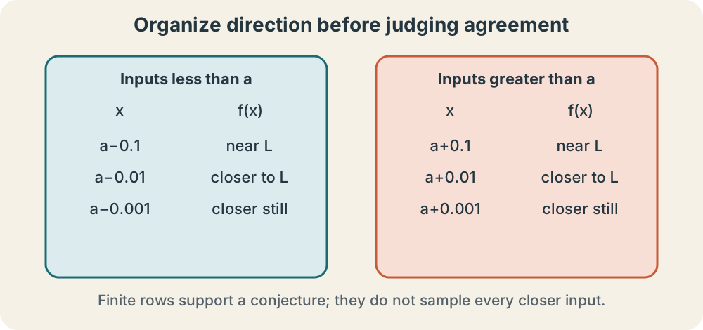
For $f(x)=\frac{x^2-1}{x-1}$ near one, values at $0.9$, $0.99$, $1.01$, and $1.1$ are generated by the nearby rule $x+1$. They approach two from both sides. The table supports $\lim_{x\to1}f(x)=2$ even though the original formula is undefined at one. Factoring proves the exact nearby equivalence that the decimals only illustrate.

A finite table cannot sample every closer input. An oscillating function may coincide with a proposed value at every chosen row and behave differently between them. Adding rows improves evidence but does not convert finite observation into proof. The statement “the table suggests” is mathematically honest. Proof requires control of all sufficiently nearby allowed inputs.

Algebra can reveal exact nearby structure

Direct substitution is a diagnostic, not the definition of a limit. If substitution produces an ordinary value and continuity is known, it may complete the calculation. If it produces $\frac00$, the form signals that nearby structure must be examined. Factoring, rationalizing, or combining fractions can reveal an equivalent expression on a punctured neighborhood. Original restrictions must remain stated.

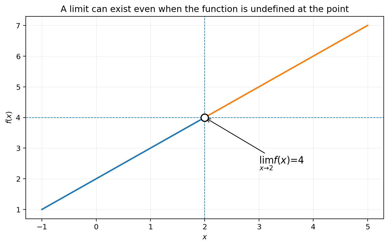
For $\frac{x^2-4}{x-2}$, factoring yields $x+2$ for $x\ne2$. Because the expressions agree at every nearby allowed input, they share the same limit at two. The simpler expression approaches four. This reasoning is stronger than a short table because it controls the whole punctured neighborhood. It does not fill the original hole.

Not every indeterminate form is resolved by the same technique. Polynomial differences invite factoring, radical differences often invite conjugates, and nested fractions need common denominators. The goal is local equivalence, not ritual simplification. Every algebraic step should answer why the transformed expression preserves nearby values. Method choice comes from structure.

Three ways a finite limit can fail

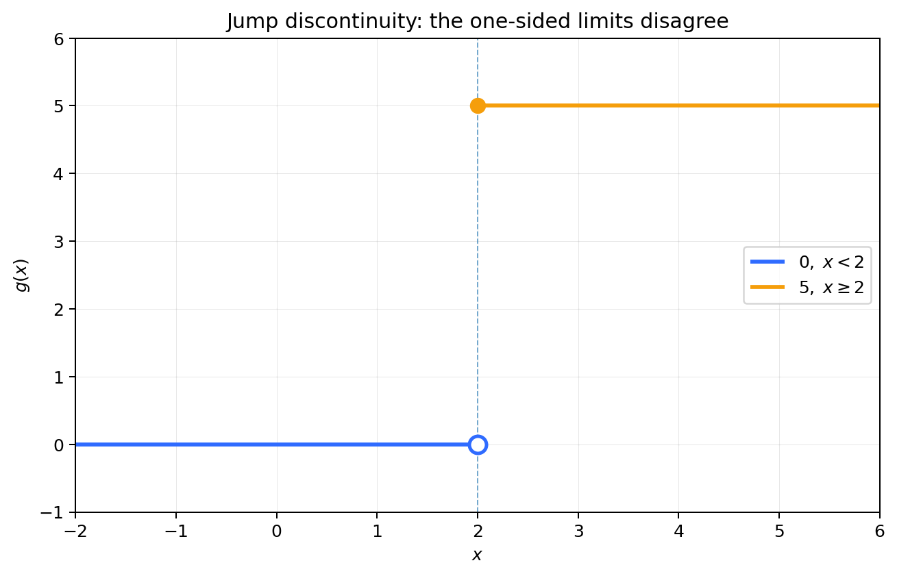
A jump occurs when outputs from opposite sides settle toward different finite values. Each side may be perfectly stable, yet no single number describes both. Assigning a point value at the target cannot repair the surrounding disagreement. The failure belongs to the neighborhood. One-sided notation will make the two destinations explicit.

Unbounded behavior occurs when output magnitude grows beyond every finite bound. A vertical asymptote often signals this behavior, although signs can differ by direction. Infinity is not a real output value reached by the function. Writing a finite limit is therefore incorrect. Extended notation can describe the growth after directions are analyzed.

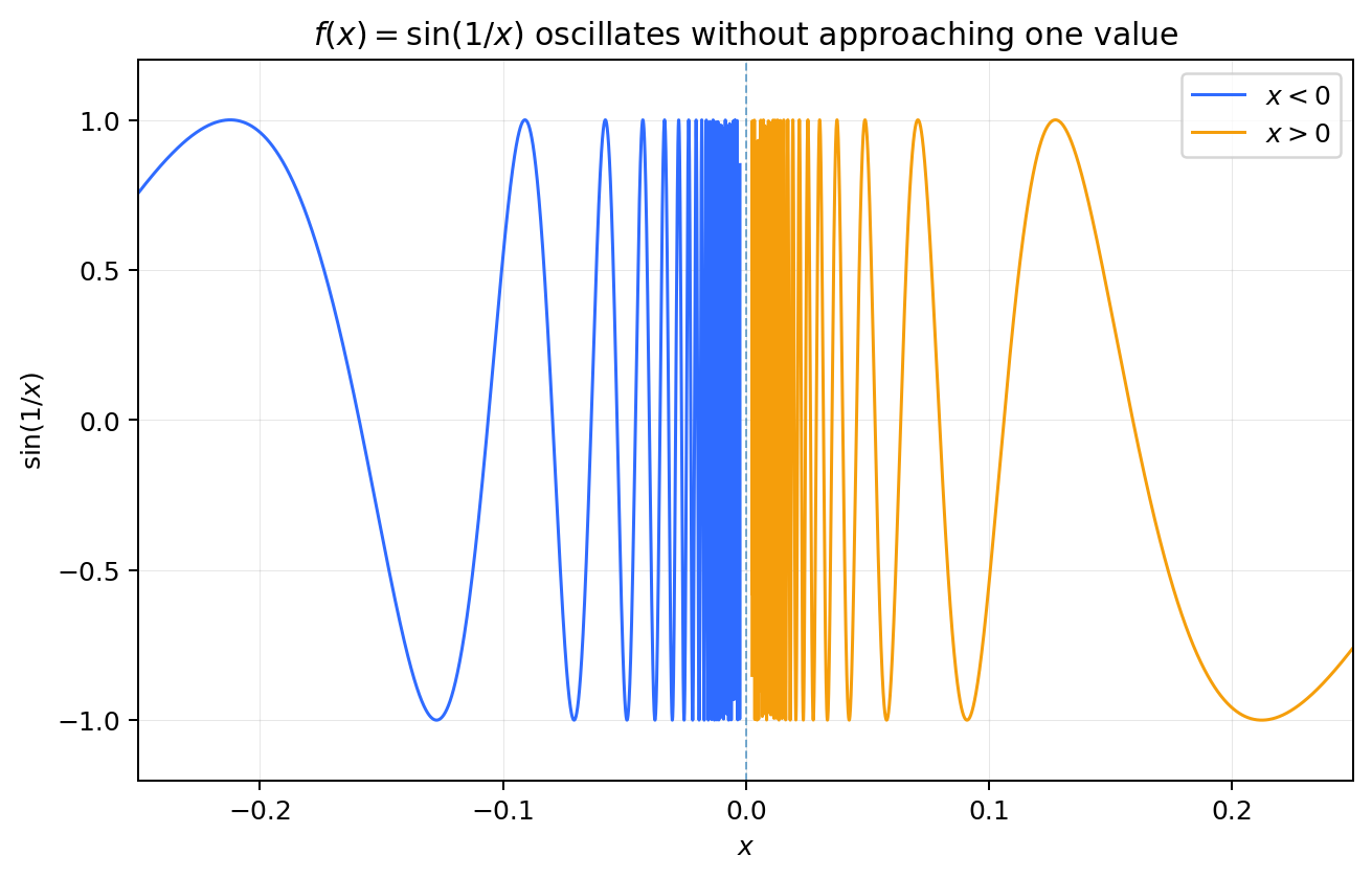
Oscillation occurs when outputs keep visiting incompatible values instead of settling. The function $\sin\left(\frac1x\right)$ remains between negative one and one but oscillates increasingly rapidly near zero. Boundedness alone does not guarantee a limit. Different input sequences can produce different output destinations. Failure does not require a jump or asymptote.

Evidence, conjecture, and proof

A conjecture is a proposed conclusion supported by observed structure. “The table suggests the limit is four” accurately describes finite evidence. “The last three decimals agree, so the limit is proven” overstates it. A proof must control every sufficiently nearby allowed input. Limit laws and epsilon-delta arguments will provide such control in later lessons.

Counterexamples test universal claims efficiently. The removable-hole example refutes “undefined point implies no limit.” A reassigned point refutes “existing limit must equal the function value.” The oscillating example refutes “bounded nearby outputs guarantee a limit.” One valid counterexample defeats a universal statement. Constructing it is a core reasoning skill.

Representation choice should match the claim. Graphs reveal spatial structure, tables estimate numerical destinations, algebra establishes exact nearby equivalence, and theorems transfer known guarantees. Strong work may coordinate several representations without pretending they contribute identical evidence. Agreement across forms raises confidence. Proof status still depends on the strongest valid argument.

Synthesis and transition

Create a two-sided table for $g(x)=\frac{x^2-9}{x-3}$ near three. State what the table suggests and then justify the result algebraically. Record the original restriction before cancellation. Sketch the graph with its missing point. Explain which statement comes from each representation and which one constitutes exact justification.

Next classify three proposed graphs: one with a jump, one with a vertical asymptote, and one with rapid bounded oscillation. For each, describe the nearby outputs without writing only “DNE.” State what evidence a sparse table might hide. Construct one misleading table for an oscillatory case. Then explain why the table remains evidence rather than proof.

Finite-limit reasoning requires both a clear claim and calibrated evidence. Graphs, tables, and formulas can support one another, but none should be granted authority it does not possess. Jumps, unbounded growth, and oscillation defeat a finite destination in different ways. The unresolved issue is how to state directional agreement precisely. The next lesson introduces left-hand and right-hand limits and turns that agreement into an existence criterion.