Reading Graphs, Tables, and Function Models

A function may be one mathematical object, but its representations do different jobs. A graph displays shape and interval behavior. A table preserves selected observations. A symbolic model exposes exact operations and parameters. Skilled calculus students move among these forms while stating which conclusions are exact, estimated, assumed, or unsupported.

This lesson focuses on evidence discipline. You will read increasing and decreasing behavior from graphs without claiming invisible precision. You will interpret tables without inventing unsampled values. You will test symbolic models with units and contextual restrictions. You will also compare representations strategically instead of assuming one is always superior. The guiding question is: what can this representation legitimately tell us?

By the end, you should identify global and local behavior, distinguish interpolation from extrapolation, and interpret model parameters. You should explain why a sparse table cannot determine a continuous function. You should compare models using domains, units, and strategically chosen inputs. You should recognize common representation-based misconceptions. The final cooling investigation leads directly to function families and transformations.

Read global behavior from a graph

A graph represents ordered pairs $(x,f(x))$ across a domain. Horizontal position records input, vertical position records output, and axis labels supply quantities and units. An $x$-intercept occurs where $f(x)=0$, while the vertical intercept is $f(0)$ when zero belongs to the domain. Turning points, holes, jumps, and asymptotes divide behavior into meaningful intervals. These features describe collections of inputs rather than isolated evaluations.

A function is increasing on an interval when larger inputs in that interval produce larger outputs. It is decreasing when larger inputs produce smaller outputs. The phrase “the graph goes up” is incomplete unless the reading direction and interval are stated. A graph can rise visually from left to right while all its outputs remain negative. Increasing describes comparison, not sign.

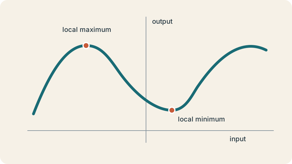
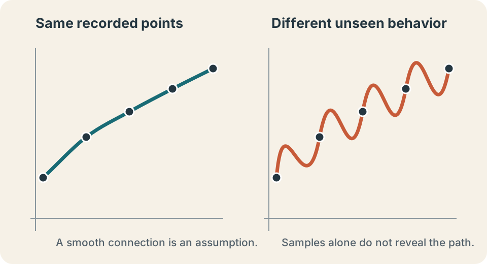
Graphical evidence has finite resolution. A smooth-looking trace may conceal a small hole, sharp corner, or rapid oscillation. Exact annotations or a known construction can establish exact facts, but a screen image usually supports estimates. A careful statement says “the graph suggests” when exactness is not warranted. Calculus uses graphs powerfully without confusing appearance with proof.

Read local and sampled behavior from a table

A table lists outputs at selected inputs and is essential when observations are measured rather than generated by a formula. Consecutive rows can reveal approximate trends, sign changes, or a possible turning region. Input spacing matters because $4$ output units across $1$ input unit is a different rate from $4$ across $10$ input units. Headings must contain units so changes and rates can be interpreted. A unitless numerical column may conceal a scientifically incomplete model.

A sparse table cannot reveal every feature between sampled inputs. Values at $x=0$, $1$, and $2$ might all be zero while a function rises sharply and returns to zero between them. Denser sampling provides more evidence but no finite table determines arbitrary behavior on a continuous interval. Interpolation estimates within the observed input span. Extrapolation extends beyond it and usually carries greater risk.

Some tables do define complete functions because the domain is finite or discrete. A fare schedule can assign one price to each listed zone. Inputs between zone numbers may be meaningless rather than merely unrecorded. Connecting those plotted points would create outputs for nonexistent inputs. Decide whether the domain is continuous, discrete, or finite before choosing a graphing convention.

Build and judge symbolic models

A symbolic model expresses output through operations on an input and parameters. Parameters remain fixed within one model but vary across a family. In $P(t)=P_0e^{kt}$, the variable $t$ changes while $P_0$ and $k$ specify the chosen member of the family. The formula supports exact evaluation and algebraic manipulation. It may still hide measurement uncertainty and the conditions under which the model is credible.

Units provide a strong coherence test. If $P$ is measured in people and $t$ in years, then $kt$ must be dimensionless, so $k$ has units of inverse years. Terms joined by addition must share units. In $d(t)=20+6t$, the initial value is $20\,\mathrm{cm}$ and the rate is $6\,\frac{\mathrm{cm}}{\mathrm{min}}$. Dimensional consistency cannot prove a model correct, but inconsistency can prove it unsuitable.

Parameters should be interpreted rather than treated as anonymous constants. In a linear model, the intercept and slope often have direct contextual meanings. In a sinusoidal model, amplitude, period, midline, and phase describe different features. In an exponential model, initial value and relative growth rate play distinct roles. The next lesson will examine how parameter changes transform entire function families.

Compare representations strategically

Two formulas can look different while defining the same function. The expressions $(x+1)^2$ and $x^2+2x+1$ agree for every real input. Vertex form makes a horizontal shift visible, while expanded form exposes polynomial coefficients. Algebraic rewriting changes which structure is easy to see without changing the assignment. Representation choice should serve the question being asked.

Conversely, similar-looking formulas can behave differently. The functions $\frac1x$ and $\frac1{x+0.01}$ place their vertical asymptotes at different inputs. Far from those inputs, their values may appear nearly equal. Surface resemblance is therefore not a reliable comparison method. State domains and test structurally important inputs.

A useful routine has four steps. First, record domains and units. Second, choose forms that reveal important features. Third, compare strategically selected inputs or intervals. Fourth, classify the relationship as equal, approximately related, or meaningfully different. This routine will later support comparison of a function with a tangent-line approximation.

Worked model: a medication reservoir

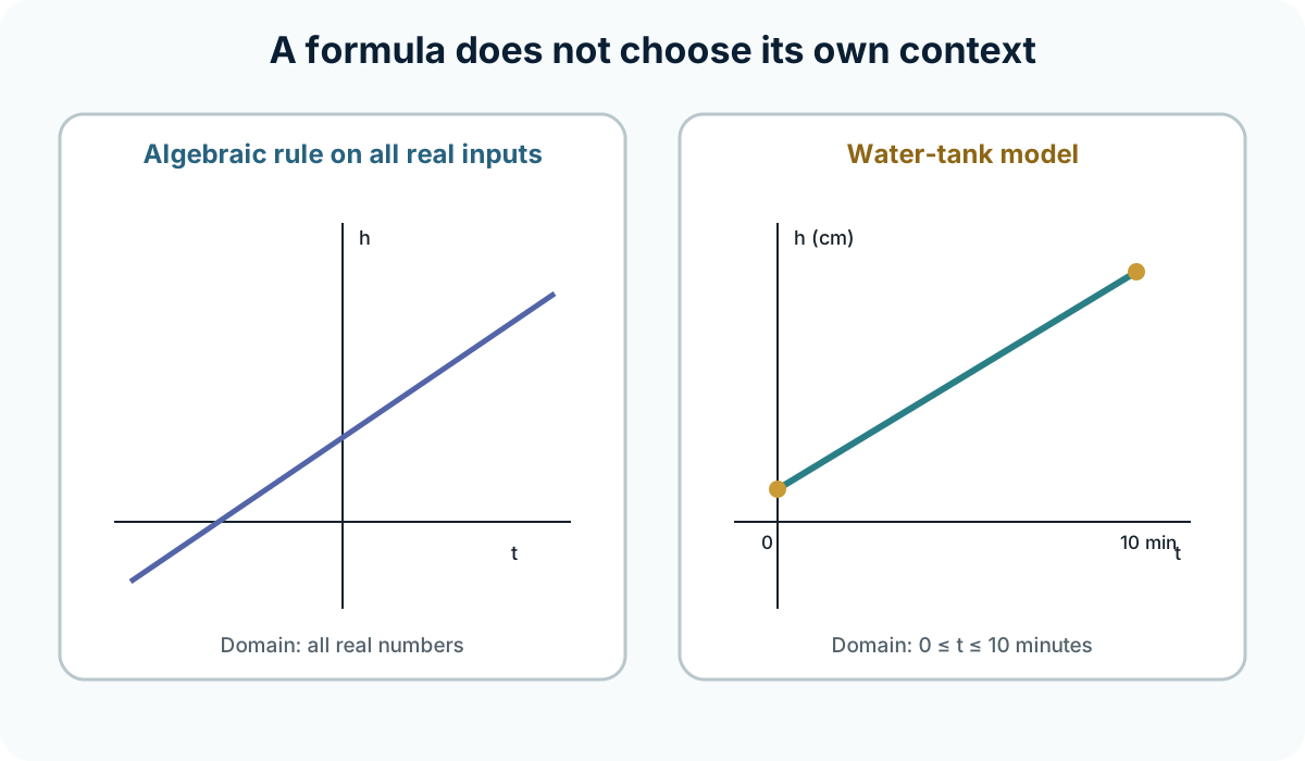
A reservoir volume is modeled by $V(t)=150-12t$, with $V$ in milliliters and $t$ in hours. Suppose the model remains valid until the volume reaches $30\,\mathrm{mL}$. Solving $150-12t=30$ gives $t=10\,\mathrm{h}$. The contextual domain is $0\le t\le10$, and the range is $30\le V\le150$ milliliters. The negative rate means volume decreases by $12\,\frac{\mathrm{mL}}{\mathrm{h}}$.

A table might include $(0,150)$, $(2,126)$, $(5,90)$, and $(10,30)$ with units in its headings. The graph is a decreasing line segment with closed endpoints. A verbal account says that the reservoir starts at $150\,\mathrm{mL}$ and loses $12\,\mathrm{mL}$ each hour for ten hours. All forms preserve the initial value, rate, domain, and units. Extending the graph past ten hours would exceed the stated model.

The formula makes exact evaluation and solving efficient. The table emphasizes selected or measured values. The graph makes decrease and endpoints visible. The verbal description supplies physical meaning and warns against extrapolation. A complete account coordinates all four rather than declaring one universally best.

Synthesis, retrieval, and transition

Close the lesson and explain one strength and one limitation of graphs, tables, formulas, and verbal models. Define interpolation and extrapolation without looking back. State why the observed range of a table may differ from the exact range of a continuous model. Then explain how units constrain addition and multiplication. Retrieval should reconstruct ideas, not merely recognize familiar words.

A technician records a component at $92\,{}^\circ\mathrm{C}$ at $0\,\mathrm{min}$, $75\,{}^\circ\mathrm{C}$ at $2\,\mathrm{min}$, $63\,{}^\circ\mathrm{C}$ at $4\,\mathrm{min}$, and $55\,{}^\circ\mathrm{C}$ at $6\,\mathrm{min}$. Identify the observed domain and range, then sketch only what the data justify. Explain what assumption is added if the points are connected. Name one additional measurement that would improve confidence in the behavior between observations.

Compare a linear cooling model with an exponential approach-to-room-temperature model. Equal time intervals in the data do not show equal temperature losses, so the linear model deserves scrutiny. Four measurements still cannot prove a unique rule. State what each family assumes and what evidence would discriminate between them. The lesson ends with an honest model comparison, and the next lesson builds the transformation language needed to study such families systematically.