Second-Order Differential Equations

A second-order differential equation relates an unknown function to its second derivative and possibly to lower derivatives, the function itself, and an input. Such equations arise naturally when acceleration, curvature, or another second rate participates in a balance. One equation can describe a moving mass, an electrical circuit, a vibrating structure, or a feedback response. The solution is not merely a formula; it is a family of trajectories shaped by internal modes, initial state, and forcing. This lesson builds a deliberate workflow for reading, solving, verifying, and interpreting the constant-coefficient linear case.

Establish the learning goals

By the end of this lesson, you should be able to classify a second-order ODE by linearity, homogeneity, and coefficient type. You will explain why two independent initial conditions normally select one solution. You will build and solve the characteristic equation for all three real-coefficient root cases. You will construct suitable trial forms for common forcing functions. You will also interpret damping, natural frequency, steady response, transients, and resonance with correct units.

The lesson emphasizes reconstruction rather than memorization. Exponential trial functions work because differentiation preserves exponential form. Complex roots produce real sine and cosine modes through Euler’s formula. Repeated roots require a second function multiplied by the independent variable. These structures can be reasoned out and verified.

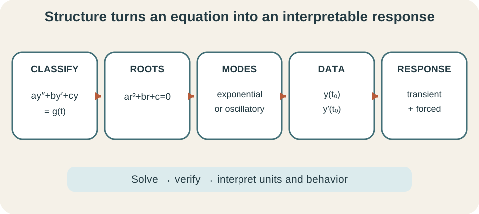
Use one workflow throughout. Normalize and classify the equation, solve the homogeneous problem, build a particular solution if forcing is present, combine the pieces, apply initial conditions, and verify. Translate constants and root types back into the physical context. Check dimensions and limiting cases before accepting a result. This sequence separates structural decisions from arithmetic.

Identify order, linearity, and forcing

A second-order ordinary differential equation contains a second derivative and no derivative of higher order. If the unknown is $y(t)$, the notation $y'$ means $\frac{dy}{dt}$ and $y''$ means $\frac{d^2y}{dt^2}$. The word ordinary means there is one independent variable. The variable is often time $t$, but it can represent position or another scalar. Order refers to the highest derivative, not to a power of $y$.

A linear second-order equation has the form $a(t)y''+b(t)y'+c(t)y=g(t)$. The coefficient functions $a$, $b$, and $c$ depend only on $t$, and $a(t)$ must not vanish on the interval being studied. The unknown and its derivatives appear only to the first power and are not multiplied together. Thus $y''+t^2y'+e^ty=\sin t$ is linear. By contrast, $y''+y^2=0$ and $yy''+y'=0$ are nonlinear.

The equation is homogeneous when $g(t)=0$ throughout the interval. It is nonhomogeneous when an external forcing function remains. Homogeneous does not mean the only solution is zero. It means the solution space is generated by internal modes with arbitrary constants. The nonhomogeneous response adds one particular forced behavior.

Read the coefficients through units

In a mechanical model $my''+cy'+ky=F(t)$, the unknown $y$ may be displacement measured in meters. Then $y'$ has units $\frac{\mathrm{meters}}{\mathrm{second}}$, and $y''$ has units $\frac{\mathrm{meters}}{\mathrm{second}^2}$. The coefficient $m$ is mass in kilograms. Therefore $my''$ has newtons because $1\,\mathrm{N}=1\,\mathrm{kilogram}\!\cdot\!\frac{\mathrm{meter}}{\mathrm{second}^2}$. This inertial term represents the force associated with acceleration.

Every term must have force units. The damping coefficient $c$ therefore has units $\frac{\mathrm{N}\!\cdot\!\mathrm{second}}{\mathrm{meter}}$, so $cy'$ is a force. The stiffness $k$ has units $\frac{\mathrm{N}}{\mathrm{meter}}$, so $ky$ is also a force. The input $F(t)$ must be measured in newtons. This unit ledger checks the model before solution begins.

Dividing by mass gives $y''+\frac{c}{m}y'+\frac{k}{m}y=\frac{F(t)}{m}$. The ratio $\frac{c}{m}$ has inverse-time units, while $\frac{k}{m}$ has inverse-time-squared units. A characteristic root must have inverse-time units because it appears in $e^{rt}$. The product $rt$ is then dimensionless. Exponential and trigonometric functions require dimensionless arguments.

Explain why two initial conditions are needed

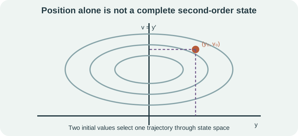
Solving a second-order equation generally introduces two independent constants. Two scalar conditions are therefore required to choose one family member under suitable existence and uniqueness conditions. In mechanics, the natural pair is displacement $y(t_0)=y_0$ and velocity $y'(t_0)=v_0$. Position alone cannot distinguish motion left, right, or momentarily at rest. The same position can lead to different future trajectories.

The state-space explanation makes this requirement concrete. Define $v=y'$. Then the second-order equation becomes two first-order equations for the state pair $(y,v)$. One initial displacement and one initial velocity specify a point in this two-dimensional state space. Repeating the same displacement condition does not add an independent state coordinate.

Boundary conditions can instead specify information at different independent-variable values. For example, $y(0)=0$ and $y(L)=0$ may describe a supported shape. Boundary-value problems can have no solution, one solution, or multiple solutions depending on the equation and values. The two-condition count remains a guide, but placement matters. Always satisfy the conditions belonging to the actual problem.

Build the characteristic equation

Consider the homogeneous constant-coefficient equation $ay''+by'+cy=0$, with $a\ne0$. Try $y=e^{rt}$ because derivatives preserve its form. Differentiation gives $y'=re^{rt}$ and $y''=r^2e^{rt}$. Substitution produces $(ar^2+br+c)e^{rt}=0$. Since $e^{rt}$ never equals zero, the factor $ar^2+br+c$ must vanish.

The algebraic equation $ar^2+br+c=0$ is the characteristic equation. Its roots determine functions that solve the differential equation. The symbol $r$ has inverse-independent-variable units in an applied model. Root real parts govern exponential growth or decay. Imaginary parts govern oscillation.

This method works because the differential operator acts on an exponential by scalar multiplication. The derivative operation becomes multiplication by $r$, and the second derivative becomes multiplication by $r^2$. The differential problem is therefore converted into a polynomial root problem. After roots are found, the resulting functions must still be combined and fitted to conditions. Algebra supplies modes, not the complete initial-value solution by itself.

Solve the distinct-real-root case

If the characteristic equation has distinct real roots $r_1$ and $r_2$, the homogeneous solution is $y_h=C_1e^{r_1t}+C_2e^{r_2t}$. The subscript $h$ denotes homogeneous response. The functions are linearly independent because their rates differ. Constants $C_1$ and $C_2$ are determined by conditions. Each exponential is called a mode.

For $y''+3y'+2y=0$, the characteristic equation is $r^2+3r+2=0$. Factoring gives $(r+1)(r+2)=0$, so roots are $-1$ and $-2$ per unit time. The family is $y=C_1e^{-t}+C_2e^{-2t}$. Both modes decay because both roots are negative. Their different decay rates make them independent modes.

The negative-one mode decays more slowly and typically dominates at long times when its coefficient is nonzero. This does not mean the negative-two mode is absent initially. Their sum can cross zero or change direction depending on constants. Initial conditions determine the mode mixture. Root inspection predicts asymptotic behavior before constants are calculated.

Solve the repeated-root case

If the characteristic polynomial has one repeated real root $r$, the function $e^{rt}$ provides only one solution direction. A second independent solution is $te^{rt}$. The homogeneous family is $y_h=(C_1+C_2t)e^{rt}$. The factor $t$ is required by the repeated algebraic structure. Using two copies of the same exponential would not produce two independent constants.

For $y''+4y'+4y=0$, the characteristic equation is $r^2+4r+4=(r+2)^2=0$. The repeated root is $r=-2$. Therefore $y=(C_1+C_2t)e^{-2t}$. Both terms decay for large positive time despite the factor $t$. Exponential decay eventually dominates polynomial growth.

Verification explains the second form. Differentiate $te^{rt}$ using the product rule and substitute it into the operator when $r$ is a repeated root. The extra terms cancel because both the characteristic polynomial and its derivative vanish at that root. This reasoning generalizes to higher multiplicities. The multiplied power of $t$ supplies missing independent modes.

Convert complex roots into real solutions

If roots are $r=\alpha\pm i\beta$, where $i^2=-1$, complex exponentials appear. Euler’s formula $e^{i\beta t}=\cos(\beta t)+i\sin(\beta t)$ converts them into real functions. The real homogeneous solution is $y_h=e^{\alpha t}[C_1\cos(\beta t)+C_2\sin(\beta t)]$. The real part $\alpha$ sets the envelope. The magnitude $|\beta|$ sets angular frequency.

For $y''+4y=0$, the characteristic equation is $r^2+4=0$, giving $r=\pm2i$. Thus $\alpha=0$ and $\beta=2\,\frac{\mathrm{radians}}{\mathrm{second}}$ when time is seconds. The family is $y=C_1\cos(2t)+C_2\sin(2t)$. With no real exponential factor, amplitude remains constant in the ideal model. Initial conditions determine the amplitude and phase encoded by the two constants.

The oscillation period is $T=\frac{2\pi}{|\beta|}$. For $\beta=2\,\frac{\mathrm{radians}}{\mathrm{second}}$, the period is $\pi\,\mathrm{seconds}$. Radians are dimensionless in calculus, while the frequency unit communicates timing. Sine and cosine repeat after a phase increase of $2\pi$. Root geometry therefore becomes observable oscillation.

Apply initial conditions systematically

Begin with the full solution family and compute its derivative before substituting values. For $y=C_1e^{-t}+C_2e^{-2t}$, differentiation gives $y'=-C_1e^{-t}-2C_2e^{-2t}$. Suppose $y(0)=3$ and $y'(0)=-4$ in compatible units. Substitution gives $C_1+C_2=3$ and $-C_1-2C_2=-4$. This is a two-equation linear system.

Solving yields $C_2=1$ and $C_1=2$. The particular initial-value solution is $y=2e^{-t}+e^{-2t}$. The coefficients carry the unit of $y$ because the exponentials are dimensionless. If $y$ is displacement, both constants have length units. The derivative automatically has length-per-time units.

Verify both requirements. Substituting into the differential equation confirms that each mode and their sum satisfy it. Evaluating at zero gives $y(0)=2+1=3$. Differentiating and evaluating gives $y'(0)=-2-2=-4$. A correct constant calculation must pass all checks.

Interpret damping through root types

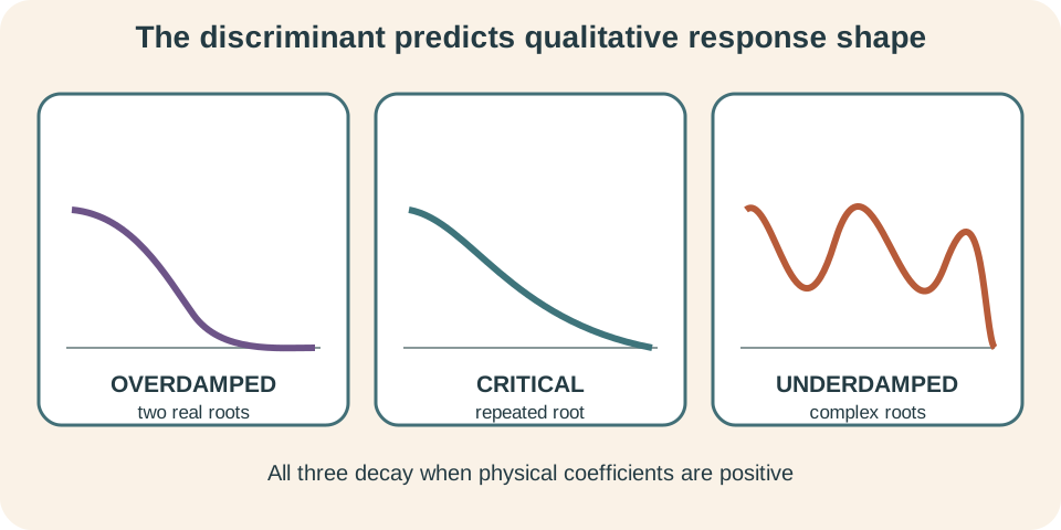
The free spring–mass–damper equation is $my''+cy'+ky=0$ with positive $m$, nonnegative $c$, and positive $k$. Its characteristic discriminant is $c^2-4mk$. If $c^2>4mk$, two distinct negative real roots produce overdamped decay. If $c^2=4mk$, a repeated root produces critical damping. If $c^2<4mk$, complex roots produce underdamped oscillation with a decaying envelope.

Overdamping returns toward equilibrium without oscillating but more slowly than the critical boundary in a common settling-time sense. Critical damping gives the fastest nonoscillatory ideal response. Underdamping crosses equilibrium repeatedly while amplitude decays. These labels describe roots and response shape. They do not state that every trajectory is visually identical within one category.

Define natural angular frequency $\omega_n=\sqrt{\frac{k}{m}}$ and damping ratio $\zeta=\frac{c}{2\sqrt{mk}}$. The ratio $\zeta$ is dimensionless. Values greater than one are overdamped, one is critically damped, and between zero and one are underdamped. Dimensionless parameters make comparisons across systems easier. Original units remain necessary when returning to physical predictions.

Separate transient and steady forced response

For $ay''+by'+cy=g(t)$, a general solution is $y=y_h+y_p$. The homogeneous term $y_h$ solves the zero-input equation and carries the initial-condition freedom. A particular solution $y_p$ is any one function satisfying the full forced equation. Linearity makes the sum valid. Different particular solutions differ by a homogeneous solution but generate the same complete family.

In a stable damped system, the homogeneous response often decays and is called the transient. The particular response associated with persistent forcing often remains and is called the steady-state response. These terms describe behavior over time rather than two unrelated equations. Initial conditions affect the transient coefficients. Forcing determines the persistent pattern.

The decomposition supports interpretation. A circuit may forget its initial capacitor voltage while continuing to respond to a sinusoidal source. A suspension may settle from an initial displacement but continue vibrating under periodic road input. A stable structure’s free modes decay while driven motion persists. The mathematical split mirrors these physical stories.

Choose trials for undetermined coefficients

The method of undetermined coefficients applies to constant-coefficient linear equations with forcing built from polynomials, exponentials, sines, cosines, and finite products of these forms. Choose a trial with the same derivative-stable family as the forcing. For $g(t)=Ke^{\lambda t}$, try $y_p=Ae^{\lambda t}$. For a polynomial of degree $n$, try a general polynomial of degree $n$. For $K\cos\omega t$, include both $A\cos\omega t+B\sin\omega t$ because differentiation mixes them.

Substitute the full trial and solve algebraically for its coefficients. Do not apply initial conditions to $y_p$ alone. Conditions belong to $y_h+y_p$. The method may fail if the coefficient functions vary with time or forcing lies outside the allowed families. Variation of parameters or transforms provide broader alternatives.

Before substitution, compare the trial with the homogeneous solution. If any trial term duplicates a homogeneous mode, multiply the entire trial by the smallest power of $t$ that restores independence. This resonance correction is structural rather than optional. Without it, substitution may collapse to an impossibility such as zero equaling a nonzero forcing. The characteristic roots reveal the required correction.

Work a nonresonant forced example

Solve $y''+3y'+2y=4$. The homogeneous roots are negative one and negative two, so $y_h=C_1e^{-t}+C_2e^{-2t}$. Constant forcing suggests the trial $y_p=A$. Then $y_p'=0$ and $y_p''=0$. Substitution gives $2A=4$, so $A=2$.

The complete family is $y=C_1e^{-t}+C_2e^{-2t}+2$. The constant two is the steady equilibrium under the constant input. Both exponential transients decay. Therefore every solution approaches two as $t$ increases when coefficients remain as modeled. This long-term limit can be predicted from root signs and the particular solution.

Suppose $y(0)=0$ and $y'(0)=0$. The conditions give $C_1+C_2=-2$ and $-C_1-2C_2=0$. Solving yields $C_1=-4$ and $C_2=2$. The initial-value solution is $y=-4e^{-t}+2e^{-2t}+2$. Direct substitution verifies the equation and both initial conditions.

Understand resonance through overlap

Consider the undamped equation $y''+\omega_0^2y=F_0\cos(\omega t)$. The homogeneous frequency is $\omega_0$. When $\omega\ne\omega_0$, a bounded sinusoidal particular solution generally exists in the ideal model. Its amplitude grows as the forcing frequency approaches the natural frequency. The denominator in the coefficient formula becomes small.

When $\omega=\omega_0$, the ordinary sine-cosine trial overlaps the homogeneous space. Multiplying by $t$ produces a particular response whose envelope grows linearly. This is ideal mathematical resonance. Energy is added coherently cycle after cycle. The unbounded growth reflects the absence of damping and nonlinear limits.

Real systems contain damping, nonlinear stiffness, finite forcing duration, or failure limits. Damping makes the steady amplitude finite and shifts details of the response peak. Resonance still matters because large responses can occur near a system frequency. Engineers therefore identify modal frequencies and damping before operating or designing structures. The ideal equation is a foundation rather than a complete safety model.

Connect the equation to a first-order system

Let $x_1=y$ and $x_2=y'$. Then $x_1'=x_2$. If $ay''+by'+cy=g(t)$, solve for $y''$ to obtain $x_2'=\frac{g(t)-bx_2-cx_1}{a}$. The second-order scalar equation becomes two coupled first-order equations. The state vector is $\mathbf x=(x_1,x_2)^T$.

For the homogeneous constant-coefficient case, write $\mathbf x'=A\mathbf x$ with matrix $A=\begin{bmatrix}0&1\\-\frac{c}{a}&-\frac{b}{a}\end{bmatrix}$. The eigenvalues of $A$ are exactly the roots of $ar^2+br+c=0$. Characteristic roots and eigenvalues are two views of the same modes. This connects differential-equation methods with linear algebra. Their eigenvectors describe corresponding state-space directions.

The system form supports numerical solvers and phase-plane analysis. A point $(y,y')$ records complete state. Equilibria, direction fields, and trajectories become geometric. Higher-order equations can be reduced similarly by adding derivative variables. State dimension equals differential order under the usual explicit form.

Verify formulas and solution domains

Verification begins by differentiating the candidate twice. Substitute $y$, $y'$, and $y''$ into the original equation rather than only its characteristic polynomial. Simplify to the stated forcing. Then check every initial or boundary condition. This process catches sign, coefficient, and trial-form errors.

The solution interval must also be stated when coefficients or forcing have singularities. A constant-coefficient equation is defined for all real $t$, but an initial-value model may be physically credible only over a limited range. If the leading coefficient $a(t)$ vanishes, solving for $y''$ may fail there. Existence and uniqueness theorems require appropriate coefficient continuity. Algebraic formulas do not erase domain restrictions.

Use qualitative checks alongside substitution. Stable negative-real-part roots should not produce growing free modes. An undamped oscillator should conserve ideal energy in the absence of forcing. Units of each term must match. Limiting cases such as zero damping or zero forcing should recover known simpler behavior.

Diagnose common solution errors

One error uses one initial condition for a second-order initial-value problem and then claims a unique solution. Another applies conditions before adding the particular solution. Both lose necessary state information. Keep two arbitrary constants until the complete family is assembled. Apply the conditions to the full expression.

Repeated roots require $te^{rt}$, and complex roots require both sine and cosine real modes. Omitting either form loses an independent solution. A forcing trial must include every derivative-coupled partner, such as sine with cosine. When overlap occurs, multiply by a suitable power of $t$. These rules all protect linear independence.

Other mistakes drop units from coefficients, confuse natural frequency with ordinary cycles-per-time frequency, or interpret every oscillation as resonance. Angular frequency has radians per time, while ordinary frequency is $f=\frac{\omega}{2\pi}$. Resonance concerns forcing near a supported system mode. Oscillation can occur freely without forcing at all. Naming the source of an oscillation prevents that conceptual confusion.

Practice the full workflow

Solve $y''-5y'+6y=0$ and classify its roots. Apply $y(0)=1$ and $y'(0)=0$. Predict long-term behavior before calculating constants. Verify the final solution in the differential equation. Explain which root controls the largest-time response.

For $2y''+8y'+8y=0$, find the characteristic roots and damping category. Write the homogeneous family. State which two initial conditions would define a mechanical motion problem. If time is measured in seconds, give root units. Explain why the second mode contains $t$.

Choose a particular-solution trial for each forcing in $y''+4y=g(t)$: $g(t)=3t+1$, $g(t)=e^t$, and $g(t)=\cos2t$. Identify which case requires a resonance correction. State the corrected trial form. Explain why cosine forcing requires a sine term in the general trial. For each choice, connect the trial family to its behavior under differentiation.

Solutions and reasoning

The characteristic equation factors as $(r-2)(r-3)=0$, so $y=C_1e^{2t}+C_2e^{3t}$. Conditions give $C_1+C_2=1$ and $2C_1+3C_2=0$. Thus $C_1=3$ and $C_2=-2$, giving $y=3e^{2t}-2e^{3t}$. Direct differentiation verifies the equation and conditions. The positive root three produces the fastest-growing mode and dominates when its coefficient is nonzero.

Dividing by two gives $y''+4y'+4y=0$, whose characteristic equation $(r+2)^2=0$ has repeated root $-2\,\frac{1}{\mathrm{second}}$. The response is $(C_1+C_2t)e^{-2t}$ and is critically damped in the normalized spring–mass interpretation. Suitable conditions are displacement $y(0)=y_0$ and velocity $y'(0)=v_0$. The factor $t$ creates a second linearly independent function. Two copies of $e^{-2t}$ would span only one mode.

For $3t+1$, try $At+B$. For $e^t$, try $Ae^t$. For $\cos2t$, the ordinary trial $A\cos2t+B\sin2t$ overlaps the homogeneous solution because roots are $\pm2i$. Multiply by $t$ to use $t[A\cos2t+B\sin2t]$. Sine is included because differentiating cosine produces sine and vice versa.

Carry second-order reasoning forward

Constant-coefficient second-order equations convert derivative structure into characteristic roots. Root type determines growth, decay, oscillation, and repeated-mode behavior. Initial conditions choose a mode combination. Forcing adds a particular response. Resonance reveals what happens when forcing overlaps an internal mode.

Systems and phase planes will express the same dynamics through a two-component state. Eigenvalues and eigenvectors will interpret characteristic roots as modal directions. Numerical methods will approximate trajectories when coefficients or forcing resist closed forms. Laplace transforms will handle inputs and initial data through another representation. The core structural reading remains useful in each extension.

Keep the workflow visible: classify, solve the homogeneous equation, choose and correct a forcing trial, combine, apply conditions, verify, and interpret. Explain every symbol and unit. Inspect roots before doing extensive arithmetic. A complete solution tells both how the function is built and what its behavior means. That dual account is the goal of second-order analysis.