Slope Fields and Euler’s Method

A first-order differential equation specifies a local rate of change rather than handing us a completed function. That rate can be displayed geometrically as a field of short tangent segments or followed numerically through a sequence of small steps. Slope fields and Euler’s method are therefore two views of the same instruction. One helps us see the family of possible solution curves, while the other constructs approximate values for a particular initial condition. Together they teach an essential modeling habit: use local information carefully, and then check whether the resulting global story is credible.

Learning objectives and the local-to-global idea

By the end of this lesson, you will be able to construct and interpret a slope field for an equation of the form $y'=F(t,y)$. You will identify nullclines, equilibrium solutions, increasing and decreasing regions, and qualitative stability. You will derive Euler’s update from a tangent-line approximation and organize repeated steps in a table. You will distinguish local truncation error from accumulated global error and explain how step size affects both accuracy and numerical stability. You will also preserve units and verify a computation against geometric and analytical evidence.

The notation $y'=F(t,y)$ says that the derivative of an unknown function $y(t)$ is determined by the current independent variable $t$ and current state $y$. The prime in $y'$ denotes differentiation with respect to $t$, so it is equivalent to $\frac{dy}{dt}$. At every point $(t,y)$ where $F$ is defined, the equation assigns one slope. A solution curve is a function whose tangent slope agrees with that assigned value at every point it visits. The equation is thus a local rule that constrains an entire curve.

This distinction between local and global information organizes the lesson. A slope field samples the local rule at many points before any initial condition is chosen. An initial condition selects one curve from the family compatible with that field. Euler’s method walks approximately along that selected curve by replacing a small curved segment with a straight tangent step. The quality of the global approximation depends on how accurately those local steps represent the changing slope.

Construct a slope field from the differential equation

To construct a slope field for $y'=F(t,y)$, choose a grid of points in the $t$-$y$ plane. At each point $(t,y)$, evaluate the number $F(t,y)$ and draw a short segment with that slope. A positive value produces a segment rising from left to right, a negative value produces a falling segment, and zero produces a horizontal segment. The segment’s location records the inputs, while its tilt records the derivative. Its length is kept short and usually standardized so that slope rather than magnitude dominates the display.

For the equation $y'=t-y$, the point $(1,3)$ receives slope $1-3=-2$. A segment there falls two vertical units for each one horizontal unit in its local direction, although the drawn segment may be scaled smaller. At $(1,1)$ the slope is zero, and at $(1,-1)$ the slope is two. Repeating the calculation across a grid reveals a coherent directional pattern. The field does not connect the segments because no initial condition has yet selected a particular solution.

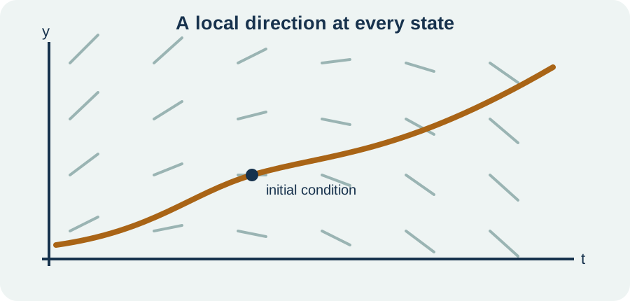
Slope fields are qualitative models rather than exact drawings of every solution. Grid spacing, segment length, and plotting range affect how much structure can be seen. A coarse grid may hide rapid changes or singular behavior. A field should therefore be labeled with its equation, axes, and scale. Visual evidence becomes trustworthy only when its sampling choices are understood.

Read solution behavior without solving explicitly

A solution increases wherever the field slopes upward and decreases wherever it slopes downward. Horizontal segments mark points where the instantaneous derivative is zero, but they do not automatically form equilibrium solutions. Concavity can be inferred by following a possible trajectory and observing whether its slopes increase or decrease along the motion. A solution passing through a field must remain tangent to nearby segments. It cannot arbitrarily jump from one directional pattern to another.

An isocline is a curve along which the slope $F(t,y)$ has a constant value. For $y'=t-y$, the zero-slope isocline satisfies $t-y=0$, so it is the line $y=t$. More generally, the isocline for slope $c$ satisfies $F(t,y)=c$. Isoclines organize a field into bands of comparable direction. They are construction aids and qualitative boundaries, not usually solution curves themselves.

Initial conditions determine which part of the field matters. The condition $y(t_0)=y_0$ specifies the point $(t_0,y_0)$ through which the selected solution must pass. Under appropriate existence and uniqueness conditions, exactly one local solution passes through that point. Two distinct solution curves then cannot cross at an ordinary point, because the crossing would assign two futures to the same initial condition. A hand-drawn curve that violates the field or crosses another unique solution has failed a structural check.

Find equilibria and interpret stability

For an autonomous equation $y'=f(y)$, the slope depends only on the state $y$ and not explicitly on time. An equilibrium occurs at a constant value $y=y_*$ satisfying $f(y_*)=0$. Because its derivative is zero at all times, the horizontal function $y(t)=y_*$ is an exact solution. In the slope field, every segment along that horizontal level is flat. Equilibria should be identified before algebraic steps divide by expressions that might equal zero.

Consider the logistic-type equation $y'=y(2-y)$. Its equilibria are $y=0$ and $y=2$ because either factor can make the product zero. Between zero and two, both factors are positive, so solutions increase. Above two, the second factor is negative, so solutions decrease. Below zero, the product is negative, so solutions decrease farther from zero.

The equilibrium $y=2$ attracts nearby solutions from both sides and is stable in this qualitative sense. The equilibrium $y=0$ repels positive nearby solutions and is unstable on that side. A phase line compresses this analysis by placing arrows on the $y$-axis according to the sign of $f(y)$. The corresponding slope field expands the same sign information across time. Stability conclusions can often be reached without an explicit solution formula.

Derive Euler’s method from a tangent line

At a known point $(t_n,y_n)$, the differential equation gives the current slope $F(t_n,y_n)$. A tangent-line approximation predicts nearby values by $y(t_n+h)\approx y_n+hF(t_n,y_n)$. The symbol $h$ is the step size, representing the horizontal change in the independent variable. The product $hF(t_n,y_n)$ is the predicted vertical change. Adding that change to $y_n$ produces the next approximate state.

Euler’s method formalizes this process as $t_{n+1}=t_n+h$ and $y_{n+1}=y_n+hF(t_n,y_n)$. The subscript $n$ labels the current numerical step rather than a derivative or exponent. The value $y_n$ approximates the true solution value $y(t_n)$. The slope is always evaluated at the current numerical point for forward Euler’s method. Once the next point is found, the method reevaluates the slope and repeats.

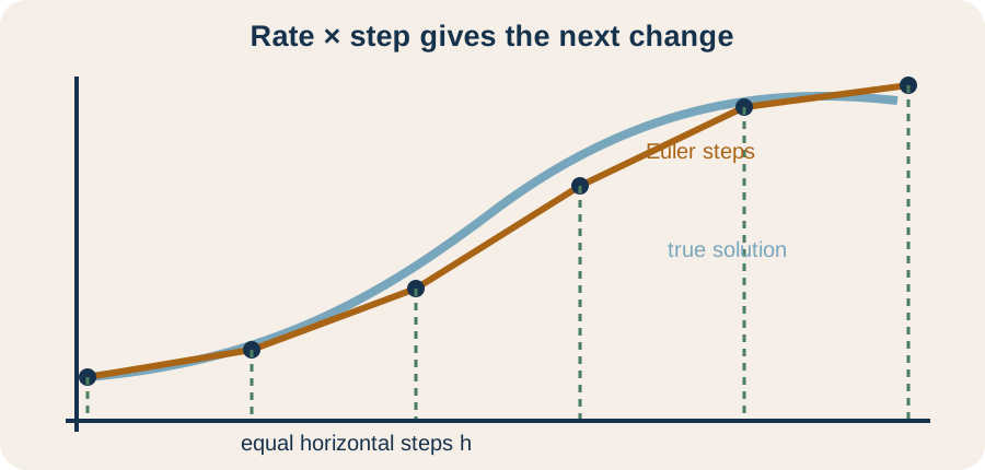
The update has the same structure as new value equals old value plus change. The change equals rate times interval, which mirrors familiar relationships such as distance equals speed times time when the speed is constant. Here the rate generally changes, so Euler treats it as constant only within one step. Smaller steps allow more frequent slope updates. This derivation explains both the method’s usefulness and its approximation error.

Execute Euler steps in a transparent table

Approximate the solution of $y'=y-t$ with $y(0)=1$ using step size $h=0.10$. At the initial point, $t_0=0$ and $y_0=1$, so the slope is $F(t_0,y_0)=1-0=1$. The first change is $(0.10)(1)=0.10$. Therefore $t_1=0.10$ and $y_1=1+0.10=1.10$. Every number should be associated with its role before the next step begins.

At the new point, the slope is $F(t_1,y_1)=1.10-0.10=1.00$. The second vertical change is again $(0.10)(1.00)=0.10$. Thus $t_2=0.20$ and $y_2=1.10+0.10=1.20$. Euler’s method reports $y(0.20)\approx1.20$. The approximation symbol $\approx$ is essential because the numerical value is not asserted to be exact.

A table with columns for $n$, $t_n$, $y_n$, $F(t_n,y_n)$, and $hF(t_n,y_n)$ makes the dependency chain visible. Complete one row using only values from that row, then carry the updated point to the next row. Do not silently replace the computed $y_n$ with an exact solution value even if one is available. The purpose is to model the numerical method’s accumulated trajectory. A table also makes recalculation with another step size straightforward.

Preserve units throughout a numerical model

Suppose $t$ is measured in seconds and $y$ is measured in meters. Then $y'=\frac{dy}{dt}$ has units of meters per second, written as the horizontal fraction $\frac{\mathrm{m}}{\mathrm{s}}$. The function $F(t,y)$ must return the same rate unit. A step size $h$ has units of seconds. Therefore $hF$ has units $\mathrm{s}\cdot\frac{\mathrm{m}}{\mathrm{s}}=\mathrm{m}$, matching the unit of $y$.

This dimensional agreement is required for the update $y_{n+1}=y_n+hF(t_n,y_n)$. Quantities can be added only when their units are compatible. If a rate is given in meters per minute while $h$ is entered in seconds, a conversion is necessary before multiplication. Writing the units beside numerical values exposes the mismatch. Units are part of the mathematical model rather than optional annotations.

For a cooling model $T'=-k(T-T_a)$, temperature $T$ and ambient temperature $T_a$ may be measured in degrees Celsius. Their difference has units of degrees Celsius, while $k$ has units of inverse time such as $\frac{1}{\mathrm{min}}$. The derivative then has units $\frac{\mathrm{^{\circ}C}}{\mathrm{min}}$. With $h=0.50\ \mathrm{min}$, the product $hT'$ has units of degrees Celsius and can update the temperature. This check also clarifies what each parameter means physically.

Distinguish local and global error

Local truncation error is the error introduced during one step when the method starts from the exact value at that step. Euler’s method uses a tangent line in place of a curved solution, so the neglected curvature produces an error typically proportional to $h^2$ for sufficiently smooth solutions. The phrase “proportional to” describes leading-order behavior as $h$ becomes small. It does not state that every problem has the same numerical constant. Smoothness assumptions and the interval of interest matter.

Global error is the difference between the exact and numerical values after many steps. On a fixed interval, approximately $1/h$ steps are required, so the one-step errors accumulate and propagate. Forward Euler’s global error is typically proportional to $h$ under standard smoothness and stability conditions. Halving $h$ therefore often roughly halves the global error. This first-order convergence is slower than the local $h^2$ behavior might initially suggest.

Error should be estimated through comparison rather than assumed from a single run. Compute the approximation with step sizes $h$ and $h/2$ and compare their values at common times. If the differences shrink by about a factor of two under further halving, the results are behaving consistently with first-order convergence. This process is called a step-refinement study. Agreement is evidence of numerical convergence, although it does not prove that the differential equation itself models reality correctly.

Predict overestimation and underestimation from concavity

Forward Euler follows the tangent line at the left endpoint of each step. If the true solution is concave upward while moving forward, the curve generally lies above its tangent line nearby. The Euler step then tends to underestimate the true value. If the solution is concave downward, the curve generally lies below its tangent, so the step tends to overestimate. These conclusions require the concavity to remain consistent over the step.

Concavity can be found by differentiating the differential equation along a solution. If $y'=F(t,y)$, then the chain rule gives $y''=F_t+F_y y'$, where $F_t$ and $F_y$ are partial derivatives. Substituting $y'=F(t,y)$ yields $y''=F_t+F_yF$. The sign of this expression along the relevant solution indicates local concavity. A visual slope field can suggest the sign by showing whether encountered slopes are becoming larger or smaller.

Do not infer overestimation merely from whether the solution is increasing or decreasing. An increasing solution may be concave upward or concave downward, and those cases produce opposite tangent-line biases. Likewise, a solution may change concavity within the interval. Compare slopes along the actual trajectory rather than across unrelated parts of the field. The geometric reason should accompany any claimed direction of error.

Understand numerical stability through a test equation

Accuracy and stability are related but distinct. A stable numerical method keeps small perturbations from growing in ways that contradict the underlying dynamics. The standard test equation $y'=\lambda y$ has exact solution $y(t)=y_0e^{\lambda t}$. When $\lambda<0$, the exact solution decays toward zero. Euler’s method should reproduce that qualitative behavior if the step size is appropriate.

Applying Euler gives $y_{n+1}=y_n+h\lambda y_n=(1+h\lambda)y_n$. The number $1+h\lambda$ is the numerical amplification factor. Decay requires its magnitude to be less than one, written $|1+h\lambda|<1$. If the factor is negative but its magnitude is below one, the approximation alternates sign while decaying. If its magnitude exceeds one, artificial oscillation or growth occurs even though the exact solution decays.

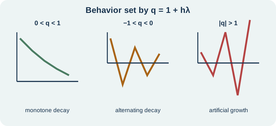
For $\lambda=-10\ \frac{1}{\mathrm{s}}$ and $h=0.30\ \mathrm{s}$, the factor is $1+(0.30)(-10)=-2$. Its magnitude is two, so numerical values double in magnitude while alternating sign. Reducing the step to $h=0.05\ \mathrm{s}$ gives factor $0.5$, which decays without sign changes. A smaller step does not repair a wrong model, but it can place the numerical method inside a stable regime. The amplification factor makes that step-size restriction explicit.

Use a four-stage verification routine

Begin with a structural check. Confirm that the equation is first order, the initial condition provides both coordinates of the starting point, and the requested direction agrees with the sign of $h$. Verify that $F(t,y)$ is defined at every numerical point used. If the field contains a singular boundary, do not step across it without analysis. A numerical table cannot override the equation’s domain.

Continue with arithmetic and dimensional checks. Recompute the slope from the current row, multiply by the signed step size, and add the resulting change to the current state. Confirm that time and state columns update together. Track units so the rate-times-step product matches the state unit. Estimate the result’s magnitude before accepting calculator output.

Finish with geometric and refinement checks. Plot several Euler points on the slope field and verify that each connecting segment follows the local direction. Compare against equilibria, monotonicity, bounds, or an exact solution when available. Repeat the calculation with a smaller step and compare values at common times. Confidence comes from several independent agreements, not from decimal precision alone.

Diagnose common mistakes and their causes

A frequent implementation error evaluates $F(t_{n+1},y_n)$ or $F(t_n,y_{n+1})$ in an otherwise forward Euler calculation. Those mixed points belong to different numerical methods or to no coherent method at all. Forward Euler evaluates both arguments at the current point $(t_n,y_n)$. Writing the slope column before the updates prevents this mistake. The formula should be read as a dependency graph rather than copied mechanically.

Another error treats an Euler value as exact or reports excessive decimal places. Numerical approximation includes discretization error even when arithmetic is performed perfectly. Roundoff error from finite precision is a separate issue and is usually smaller for introductory examples. Report enough digits to show the calculation without implying unsupported certainty. State the step size whenever giving a numerical result because accuracy depends on it.

A third error assumes that smaller steps always solve every problem. Smaller $h$ usually reduces truncation error and may improve stability, but it increases computational work and can magnify the total effect of roundoff in extreme cases. Stiff equations may require impractically small forward Euler steps. More advanced methods use better local approximations or stability properties. Method choice is part of modeling, not merely a software detail.

Practice qualitative and numerical reasoning

For $y'=t+y$ with $y(1)=2$, take two forward Euler steps using $h=0.25$. Build a table containing the current point, slope, change, and updated point. Attach units if $t$ is in seconds and $y$ is in meters. Predict from the slope field whether the solution is increasing over these steps. Explain why the approximation symbol belongs in the final statement.

For the autonomous equation $y'=y^2-1$, find all equilibrium solutions and construct a phase line. Determine the sign of the derivative in the intervals separated by those equilibria. Classify each equilibrium’s stability from both sides. Sketch a small slope field consistent with the phase line. Explain why dividing by $y^2-1$ before listing equilibria could lose valid solutions.

For $y'=-4y$ with $y(0)=1$, compare Euler step sizes $h=0.20\ \mathrm{s}$ and $h=0.60\ \mathrm{s}$ over several steps. Calculate each amplification factor and predict the numerical behavior before making a table. Compare both approximations with the exact qualitative behavior of positive exponential decay. Identify which failure is primarily about stability rather than ordinary small truncation error. Recommend a safer step and justify it using $|1+h\lambda|<1$.

Solutions and reasoning

For the first problem, the initial slope is $1+2=3\ \frac{\mathrm{m}}{\mathrm{s}}$, so the change is $(0.25\ \mathrm{s})(3\ \frac{\mathrm{m}}{\mathrm{s}})=0.75\ \mathrm{m}$. This gives $(t_1,y_1)=(1.25\ \mathrm{s},2.75\ \mathrm{m})$. The next slope is $1.25+2.75=4.00\ \frac{\mathrm{m}}{\mathrm{s}}$, and the next change is $1.00\ \mathrm{m}$. Therefore $y(1.50\ \mathrm{s})\approx3.75\ \mathrm{m}$, with the field indicating continued increase. The approximation symbol records that tangent steps replaced the curved trajectory.

For the second problem, $y^2-1=(y-1)(y+1)$ gives equilibria $y=-1$ and $y=1$. The derivative is positive below negative one, negative between negative one and one, and positive above one. Arrows therefore point upward, downward, and upward across the three intervals. The equilibrium at negative one attracts from both sides and is stable, while the equilibrium at one repels from both sides and is unstable. Dividing by the zero-producing factor would exclude both constant solutions.

For the third problem, $h=0.20\ \mathrm{s}$ gives factor $1+(0.20)(-4)=0.20$, so the numerical sequence decays without sign changes. The step $h=0.60\ \mathrm{s}$ gives factor $1+(0.60)(-4)=-1.40$, whose magnitude exceeds one. That approximation alternates sign and grows, contradicting the exact decay. The stability condition becomes $|1-4h|<1$, which requires $0<h<0.50\ \mathrm{s}$. A choice such as $h=0.10\ \mathrm{s}$ lies safely inside that interval.

Connect the method to broader numerical analysis

Euler’s method is the simplest member of a large family of time-stepping methods. Improved Euler and Runge–Kutta methods sample more slope information within a step to obtain higher accuracy. Implicit methods evaluate relationships involving the new state and can offer stronger stability for stiff problems. Adaptive algorithms change the step size in response to estimated local error. Every refinement still builds on the same local-to-global idea developed here.

Second-order differential equations can be rewritten as systems of first-order equations. A position equation involving acceleration becomes a system for position and velocity, and Euler then updates both state variables at each step. The geometric picture moves from a two-dimensional slope field to a direction field in a higher-dimensional phase space. Equilibria and stability remain central. The notation grows, but the reasoning pattern survives.

The enduring lesson is to combine representations. Use the differential equation to compute local rates, the slope field to see qualitative structure, Euler’s method to generate approximate values, and refinement to measure numerical sensitivity. Preserve domain restrictions and units throughout. An approximation becomes scientifically meaningful only when its arithmetic, geometry, and assumptions agree. No single representation supplies all of those checks by itself.