First-Order Differential Equations

A differential equation specifies how a state changes rather than giving the state directly. A first-order ordinary differential equation connects an unknown function to its first derivative with respect to one independent variable. Solving means finding a function, an interval, and any constants that make the relationship true. Classification reveals which exact method may work, while qualitative reasoning predicts behavior before calculation. This lesson develops a repeatable workflow that keeps equilibria, domains, units, and initial data visible throughout the algebra.

Identify the unknown state and independent variable

Write the unknown function explicitly before manipulating the equation. In $y'=F(t,y)$, the state is $y(t)$. The independent variable is $t$. The prime means $dy/dt$. The function $F$ supplies the rate at each allowed pair $(t,y)$.

The adjective first-order means no derivative higher than $y'$ appears. The adjective ordinary means there is one independent variable. The equation can still be nonlinear in $y$. For example, $y'=y^2-t$ is first-order and nonlinear. Classification terms describe different structural features.

Attach units at this stage. If $t$ is seconds and $y$ is metres, then $y'$ has units $\mathrm{m\,s^{-1}}$. Every term in $F(t,y)$ must have those same rate units. A unit mismatch reveals a model error before integration begins. Parameters often carry the factors needed to restore dimensional consistency.

Distinguish a differential law from its solutions

The equation $y'=2t$ is a rule for slope. Integrating gives family $y=t^2+C$. The constant $C$ can take many values. Each value shifts the curve vertically while preserving the derivative. The differential law therefore defines a family rather than one trajectory.

An initial condition such as $y(0)=3$ selects a member. Substitution gives $3=0^2+C$, so $C=3$. The resulting initial-value solution is $y=t^2+3$. Both equation and initial condition must be checked. Satisfying one without the other is incomplete.

A solution also has a domain interval. Formula $y=1/(C-t)$ solves $y'=y^2$ only where its denominator is nonzero. A singular time divides possible intervals. An initial condition selects the relevant interval containing its initial point. Ignoring that interval can turn a local solution into a false global claim.

Classify before selecting an exact method

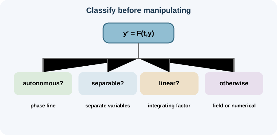
Begin by asking whether the equation is autonomous. An autonomous equation has form $y'=f(y)$ with no explicit independent variable. Then ask whether it is separable as $y'=g(t)h(y)$. Finally, check whether it is linear in form $y'+p(t)y=q(t)$. More than one answer can be yes.

Equation $y'=1-y$ is autonomous because the right side depends only on $y$. It is separable because $dy/(1-y)=dt$ away from equilibrium. It is also linear because $y'+y=1$. Multiple methods can solve it. Their agreement creates a useful check.

Equation $y'=t+y^2$ is neither autonomous nor separable in the elementary product sense. It is nonlinear because of $y^2$. The methods developed here do not provide a general elementary solution. A slope field or numerical solver may still produce insight. Classification prevents forcing an inapplicable technique.

Find equilibrium solutions before dividing

For autonomous equation $y'=f(y)$, an equilibrium is a constant solution $y(t)=y_*$ satisfying $f(y_*)=0$. The star labels a special constant value. Its derivative is zero. Substituting the constant into the original equation verifies it. Equilibria organize nearby behavior.

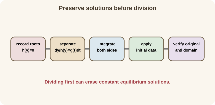
Separation often divides by a factor containing $y$. If that factor is zero at an equilibrium, division excludes the constant solution. Therefore solve $h(y)=0$ before rearranging $y'=g(t)h(y)$. Record each constant solution separately. Then solve the non-equilibrium branches under the assumption $h(y)\neq0$.

For $y'=y(2-y)$, equilibria are $y=0$ and $y=2$. Dividing by $y(2-y)$ is legal only away from those values. The separated family may approach either equilibrium without including the constant curves automatically. Adding the equilibrium solutions completes the solution set. This habit prevents a subtle loss caused by otherwise valid algebra.

Separate variables as a structured transformation

A separable equation can be written $dy/dt=g(t)h(y)$. For non-equilibrium branches with $h(y)\neq0$, rearrange to $dy/h(y)=g(t)\,dt$. The notation groups all state dependence with $dy$ and all independent-variable dependence with $dt$. Integration follows on both sides. The manipulation is justified through the chain rule and antiderivatives.

Write the integrated form $\int\dfrac{1}{h(y)}\,dy=\int g(t)\,dt+C$. One combined constant is enough because two arbitrary additive constants can be subtracted into one. Evaluate both antiderivatives carefully. Then solve explicitly for $y$ when possible. An implicit relation can still be a valid solution.

Every transformation has conditions. Division requires nonzero $h(y)$. Logarithmic antiderivatives create absolute values. Exponentiation may introduce a nonzero multiplicative constant and branch constraints. Verification against the original equation checks the result more reliably than trusting a familiar pattern.

Solve a basic exponential equation

Consider $y'=ky$, where $k$ is constant. The equilibrium $y=0$ should be recorded first. For $y\neq0$, separation gives $dy/y=k\,dt$. Integration yields $\ln|y|=kt+C$. The natural logarithm appears because its derivative is $1/y$.

Exponentiation gives $|y|=e^Ce^{kt}$. Absorb the positive factor and possible sign into one constant $A$. The solution family becomes $y=Ae^{kt}$. Allowing $A=0$ includes the equilibrium. This final parameterization is simpler than carrying an absolute value.

If $y(0)=y_0$, then $A=y_0$. The initial-value solution is $y=y_0e^{kt}$. Parameter $k$ has units inverse time so exponent $kt$ is dimensionless. Positive $k$ produces growth, while negative $k$ produces decay. Substitution gives $y'=ky_0e^{kt}=ky$, confirming the differential equation.

Solve a separable equation with time dependence

Consider $y'=3ty$. The equilibrium $y=0$ is visible from the right side. For nonzero solutions, write $dy/y=3t\,dt$. Integration gives $\ln|y|=\dfrac{3}{2}t^2+C$. Exponentiating produces $y=Ae^{3t^2/2}$.

The exponent must be dimensionless in an applied model. If $t$ has seconds, the numerical coefficient three cannot be unitless. It must supply units $\mathrm{s^{-2}}$ in the original rate coefficient $3t$. Then $(3/2)t^2$ is dimensionless. Unit analysis clarifies what an abbreviated textbook number suppresses.

Differentiate the solution to verify it. The chain rule gives $y'=Ae^{3t^2/2}(3t)$. This equals $3ty$. Setting $A=0$ returns the equilibrium. The verification checks the exponent factor and the previously separated family simultaneously.

Use partial fractions for logistic growth

The logistic equation is $dP/dt=rP\left(1-P/K\right)$. Population $P$ and carrying capacity $K$ share the same units. Therefore $P/K$ is dimensionless. Parameter $r$ has units inverse time. Equilibria occur at $P=0$ and $P=K$.

For other solutions, separate as $\dfrac{dP}{P(1-P/K)}=r\,dt$. Partial fractions decompose the state side. Integration produces logarithms of $P$ and $K-P$ on an interval where their signs are controlled. Algebra then yields $P(t)=\dfrac{K}{1+Ae^{-rt}}$. The constant $A$ is determined by initial population.

For $P(0)=P_0$ with $0<P_0<K$, substitution gives $A=(K-P_0)/P_0$. This constant is positive. As $t\to\infty$, $e^{-rt}\to0$ for positive $r$, so $P(t)\to K$. The explicit solution agrees with the phase-line prediction. The model assumes constant carrying capacity and a growth rate depending only on current population.

Write a linear equation in standard form

A first-order linear equation has standard form $y'+p(t)y=q(t)$. The coefficient of $y'$ must be one. If an equation begins as $a(t)y'+b(t)y=c(t)$, divide by $a(t)$ where $a(t)\neq0$. That division may restrict the interval. Record any excluded points.

Linearity means $y$ and $y'$ appear only to the first power and are not multiplied together. Coefficients may depend on $t$. Equation $y'+t^2y=\sin t$ is linear. Equation $y'+y^2=t$ is not. Equation $yy'=t$ is not linear in standard form.

The function $q(t)$ is often called forcing. When $q=0$, the equation is homogeneous in the first-order linear sense. The term does not mean the same thing as a homogeneous function in every area of mathematics. Context determines vocabulary. Standard form makes the coefficient and forcing roles explicit.

Derive the integrating factor

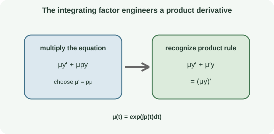
Start with $y'+p(t)y=q(t)$. Seek a nonzero function $\mu(t)$ that makes the left side a product derivative. Multiplying gives $\mu y'+\mu py=\mu q$. The product rule says $(\mu y)'=\mu y'+\mu'y$. Therefore require $\mu'=p\mu$.

Solving $\mu'/\mu=p$ gives $\mu=e^{\int p(t)\,dt}$. A multiplicative constant in $\mu$ is unnecessary because it cancels later. With this choice, the equation becomes $(\mu y)'=\mu q$. Integrate once to obtain $\mu y=\int\mu q\,dt+C$. Divide by $\mu$ to find $y$.

The method is an engineered product rule. It is not an unexplained formula. Checking $\mu'=p\mu$ validates the factor. Checking the expanded product derivative validates the transformed equation. These small checks prevent a sign error from propagating through the solution.

Solve a linear initial-value problem

Solve $y'+2y=4$ with $y(0)=1$. The equation is already in standard form with $p=2$ and $q=4$. The integrating factor is $\mu=e^{2t}$. Multiplication gives $e^{2t}y'+2e^{2t}y=4e^{2t}$. The left side is $(e^{2t}y)'$.

Integrating gives $e^{2t}y=2e^{2t}+C$. Division yields $y=2+Ce^{-2t}$. The initial condition gives $1=2+C$, so $C=-1$. Therefore $y(t)=2-e^{-2t}$. This solution approaches equilibrium two from below.

Verification gives $y'=2e^{-2t}$. Then $y'+2y=2e^{-2t}+4-2e^{-2t}=4$. Also, $y(0)=2-1=1$. Both equation and data hold. Long-term behavior agrees with the sign rule $y'=4-2y$.

Model Newton cooling as linear and separable

Newton’s cooling law is $T'=-k(T-T_{\mathrm{env}})$ for positive $k$. The environmental temperature is constant in the simplest model. The equation is autonomous and separable. Expanding gives $T'+kT=kT_{\mathrm{env}}$, so it is also linear. Multiple structures provide multiple solution routes.

Let $u=T-T_{\mathrm{env}}$. Then $u'=T'$ because the environment is constant. The equation becomes $u'=-ku$. Thus $u=u_0e^{-kt}$. Returning to temperature gives $T=T_{\mathrm{env}}+(T_0-T_{\mathrm{env}})e^{-kt}$.

Temperature difference and temperature share degree units, while $k$ has units inverse time. The exponential argument is dimensionless. If $T_0>T_{\mathrm{env}}$, the difference decays from positive values. If $T_0<T_{\mathrm{env}}$, it approaches zero from negative values. The environment is an attracting equilibrium under the model.

Analyze autonomous stability with a phase line

For $y'=f(y)$, place equilibria where $f(y)=0$ on a vertical or horizontal phase line. Determine the sign of $f$ between equilibria. Positive sign means $y$ increases with time. Negative sign means it decreases. Arrows summarize those directions.

For $y'=y(2-y)$, signs are negative below zero, positive between zero and two, and negative above two. Arrows point away from zero on both sides. Thus zero is repelling. Arrows point toward two on both sides. Thus two is attracting.

Stability conclusions do not require an explicit formula. They also help validate one. A proposed solution starting between zero and two should increase without crossing the attracting equilibrium under uniqueness conditions. A numerical trajectory that leaves this band may reflect excessive step size. Qualitative structure supplies a strong diagnostic.

Apply existence and uniqueness correctly

For initial-value problem $y'=F(t,y)$ and $y(t_0)=y_0$, continuity of $F$ near the initial point supports local existence. Continuity of partial derivative $\partial F/\partial y$ near the point is a common sufficient condition for local uniqueness. The notation means the rate at which $F$ changes with its state argument while $t$ is held fixed. These conditions are sufficient rather than necessary. They provide a dependable test, but failing the test does not by itself prove that a solution is absent or nonunique.

Uniqueness explains why two solution curves cannot cross at an ordinary point in the region. A crossing would give one initial condition two distinct solutions. The conclusion is local and depends on the theorem’s conditions. Singularities or nonsmooth rate laws can permit nonunique behavior. A slope field alone does not prove the theorem.

Existence also does not guarantee a solution for all time. A solution can blow up at finite time or reach a domain boundary. Equation $y'=y^2$ has solution $y=1/(C-t)$ on intervals excluding $t=C$. The local theorem remains compatible with finite-time singularity. Always state the solution interval.

Preserve units throughout a model

In $y'=ky$, the units of $k$ are reciprocal units of the independent variable. If time uses seconds, $k$ uses $\mathrm{s^{-1}}$. Then $ky$ has units of $y$ per second. The product $kt$ is dimensionless. Exponential functions require dimensionless arguments.

In logistic growth, $r$ has inverse-time units and $K$ has population units. The factor $1-P/K$ is dimensionless. In cooling, $k$ has inverse-time units and temperature difference has temperature units. Every right-side term matches the derivative units. These checks reveal whether parameters have been interpreted correctly.

Integration constants also have units. In $y=Ae^{kt}$, $A$ has the same units as $y$. In $\ln|y|=kt+C$, taking a logarithm of a dimensional quantity is shorthand that should really use a reference scale. The final ratio or exponential form resolves that issue. Careful modeling keeps the dimensionless structure explicit.

Verify solutions in four stages

First differentiate the proposed function. Second substitute the function and derivative into the original equation. Third check the initial condition. Fourth state a valid interval. Each stage catches a different failure.

Do not verify only the rearranged equation. Separation may have divided by a zero factor. Logarithm and exponentiation may alter domain descriptions. Solving for a square root may choose a branch. Return to the original differential law.

Also compare qualitative behavior. Check signs near equilibria. Check long-term limits. Check units. Agreement among algebra, data, domain, and behavior makes the solution credible.

Diagnose recurring method errors

One error is attempting separation when the right side is a sum that cannot be factored into $g(t)h(y)$. Another is dividing away equilibrium solutions. A third is applying an integrating factor before standardizing the coefficient of $y'$. A fourth is forgetting the integration constant. Classification and a written workflow prevent these errors.

Absolute values are often dropped too early after integrating $1/y$. Exponentiation should absorb sign into a constant only after branches are understood. Initial data then determine the constant. Domain restrictions remain. Symbolic neatness should not erase logical conditions.

Another error is treating model parameters as unitless. A number such as $0.2$ must often be $0.2\,\mathrm{h^{-1}}$. Writing units clarifies time scale. It also keeps exponents dimensionless. A correct-looking formula with a dimensional exponent is physically incomplete.

Practice a complete workflow

For $y'=3ty$, identify the equilibrium before separating. Solve the nonzero family. Include the equilibrium through the final constant. Differentiate and substitute. State the units needed for the coefficient when $t$ carries time units.

For $y'+2y=4$, identify linear standard form. Construct the integrating factor and verify its derivative. Solve for the general family. Apply a chosen initial condition. Use the autonomous sign pattern to predict the limiting value.

For $y'=y(2-y)$, find equilibria and create a phase line. Classify stability. Separate non-equilibrium branches if an explicit formula is requested. Preserve the two constant solutions. Compare the explicit behavior with the arrows.

Connect forward to slope fields and numerical methods

Exact methods apply to important structural families but not every first-order equation. Slope fields display $F(t,y)$ geometrically. Euler’s method turns the local slope into small numerical steps. Higher-order solvers sample slope more intelligently. Classification still informs expected behavior.

Equilibria and uniqueness guide numerical validation. Units guide step-size interpretation. Exact solutions provide benchmark problems for testing algorithms. Domain singularities warn where step control matters. The habits developed here carry directly into computation.

You are ready to continue when you can classify an equation, preserve equilibria, execute separation or an integrating factor, and verify the result in the original problem. You should attach units and state intervals. You should also predict stability before solving. These skills turn first-order methods into a coherent workflow. Slope fields and Euler’s method can then extend the analysis beyond convenient exact forms.