Separable ODEs Put Each Variable on Its Own Side

A first-order differential equation gives a local rate, but a separable equation has enough factor structure to convert that rate rule into integrals. The method places every state-dependent factor with the state differential and every independent-variable factor with the independent-variable differential. Integration then produces an implicit relation or explicit solution family. An initial condition selects one member of that family. The method is powerful because it joins algebra, the chain rule, integration, and qualitative dynamics.

Separation must be used carefully. Dividing by a state factor can discard constant equilibrium solutions, logarithms introduce absolute values and domain branches, and algebraic rearrangement can create formulas valid only on restricted intervals. A correct solution therefore begins with classification and equilibrium checks and ends with substitution into the original equation. Units and phase-line reasoning supply additional evidence. This article develops that complete workflow rather than treating differentials as symbols that can be moved without justification.

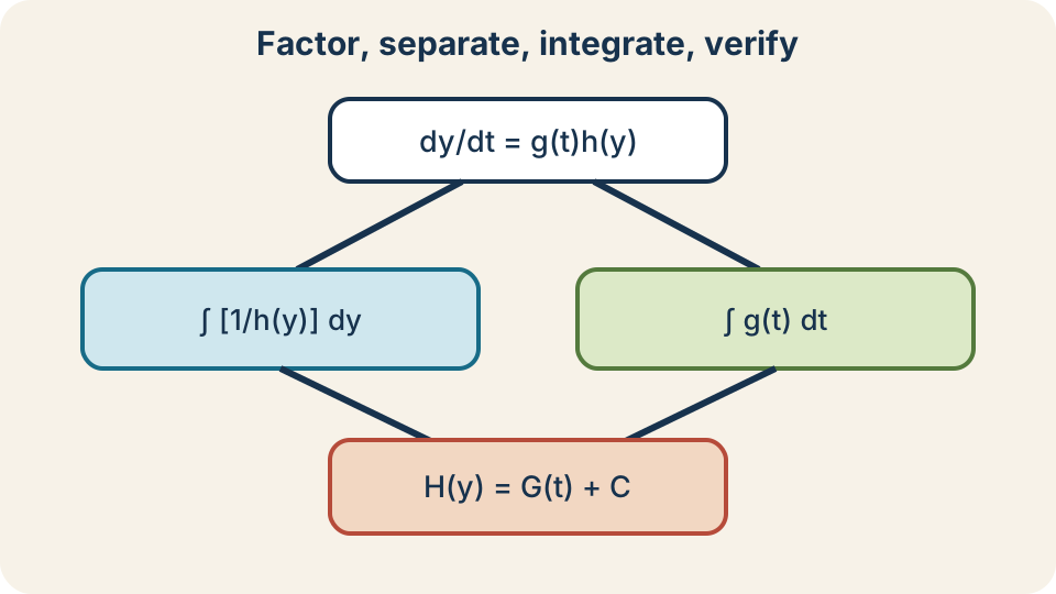
A separable rate factors into a time part and a state part. State-dependent factors are collected with $dy$. Time-dependent factors are collected with $dt$. Each side is then integrated in its own variable. The resulting relation must still be solved, restricted, and verified.

Recognize the separable structure

An equation is separable when it can be written as $\frac{dy}{dt}=g(t)h(y)$. The function $g$ depends only on the independent variable $t$. The function $h$ depends only on the state $y$. A constant may be included in either factor. The defining feature is a product of one-variable factors rather than an arbitrary mixture of $t$ and $y$.

For example, $y'=t(1+y^2)$ is separable with $g(t)=t$ and $h(y)=1+y^2$. The equation $y'=t+y$ is not separable in that form because the right side is an inseparable sum. It may be solved by a linear-equation method instead. The equation $y'=\frac{t}{y}$ is separable because it can be written $yy'=t$. Classification prevents a method from being forced onto the wrong structure.

Algebraic rewriting may reveal hidden separability. If $y'=\frac{t+1}{y-3}$, multiplication by $y-3$ gives $(y-3)\frac{dy}{dt}=t+1$. If $y'=\frac{t+y}{ty}$, the right side becomes $\frac{1}{y}+\frac{1}{t}$, which is not a product of a pure time function and pure state function. Not every rearrangement that moves some symbols creates separation. Both sides after separation must be integrable in only their own variables.

Record equilibrium solutions before dividing

For an autonomous separable equation $y'=g(t)h(y)$, any root $y^*$ of $h(y)=0$ gives a constant solution $y(t)=y^*$. Substitution confirms that its derivative is zero and the right side is also zero. These solutions are equilibria because the state does not change. They should be listed before division by $h(y)$. Division assumes the factor is nonzero.

Consider $y'=y(1-y)$. The roots of the state factor are $y=0$ and $y=1$. Therefore $y(t)=0$ and $y(t)=1$ are constant solutions. Dividing by $y(1-y)$ removes both possibilities from the algebraic branch. The nonconstant family found afterward does not replace the missing equilibria.

This issue is logical rather than cosmetic. Dividing an equation by an expression restricts attention to points where that expression is nonzero. If an initial condition lies at an equilibrium, the constant solution may be the unique solution. A final answer that omits it is incomplete. The “equilibrium first” habit prevents a common loss of valid solutions.

Separate variables with conditions visible

Where $h(y)\ne0$, rewrite $\frac{dy}{dt}=g(t)h(y)$ as $\frac{1}{h(y)}\,dy=g(t)\,dt$. The differential $dy$ is grouped with a function of $y$, and $dt$ with a function of $t$. This notation summarizes a chain-rule operation. It should not be interpreted as unrestricted fraction cancellation in every differential equation. The nonzero condition on $h$ remains in force for this branch.

Integrating gives $\int\frac{1}{h(y)}\,dy=\int g(t)\,dt$. Let $H'(y)=\frac{1}{h(y)}$ and $G'(t)=g(t)$. Then the integrated relation is $H(y)=G(t)+C$. One arbitrary constant is enough because two integration constants can be combined by subtraction. The relation may already be a useful implicit solution.

An explicit solution isolates $y$ as a function of $t$. This isolation can introduce choices, restrictions, or inverse functions. Some equations cannot be solved explicitly with elementary functions, while their implicit relations remain valid. Do not discard an implicit answer merely because it is not written as $y=$. The problem’s request determines whether further isolation is necessary.

Justify the method through the chain rule

Suppose $H'(y)=\frac{1}{h(y)}$ on a branch where $h(y)\ne0$. Along a differentiable solution, the chain rule gives $\frac{d}{dt}H(y(t))=H'(y(t))y'(t)$. Substituting the differential equation yields $\frac{1}{h(y)}g(t)h(y)=g(t)$. Therefore $\frac{d}{dt}H(y(t))=g(t)$. Integrating with respect to $t$ produces $H(y(t))=G(t)+C$.

This argument explains the familiar differential rearrangement. The symbols $dy$ and $dt$ support a concise and reliable notation because the chain rule lies underneath. They are not independent algebraic numbers in an unrestricted sense. The nonzero factor cancellation is precisely the step that excluded equilibria. Knowing the justification reveals both the method’s power and its limitation.

Verification reverses the chain-rule reasoning. Differentiate the proposed implicit or explicit relation. Use algebra to recover the original differential equation. Then confirm the initial condition and domain. A derivation without verification can conceal a lost sign, missing absolute value, or invalid branch.

Solve proportional growth and decay

Consider $y'=ky$, where constant $k$ has reciprocal-time units. The equilibrium solution is $y=0$. For nonzero states, separation gives $\frac{1}{y}\,dy=k\,dt$. Integration produces $\ln|y|=kt+C$. The absolute value appears because an antiderivative of $\frac{1}{y}$ is $\ln|y|$ on nonzero intervals.

Exponentiating gives $|y|=e^Ce^{kt}$. The positive quantity $e^C$ and a possible sign can be combined into a nonzero constant $A$, yielding $y=Ae^{kt}$. Allowing $A=0$ reincorporates the equilibrium solution in this special final form. An initial condition $y(t_0)=y_0$ gives $A=y_0e^{-kt_0}$. Equivalently, $y(t)=y_0e^{k(t-t_0)}$.

If $k>0$, nonzero magnitude grows away from zero as time increases. If $k<0$, magnitude decays toward zero. The exponent $k(t-t_0)$ must be dimensionless, so reciprocal-time units for $k$ are required. A positive initial state stays positive and a negative initial state stays negative. The explicit formula agrees with the equilibrium barrier at zero.

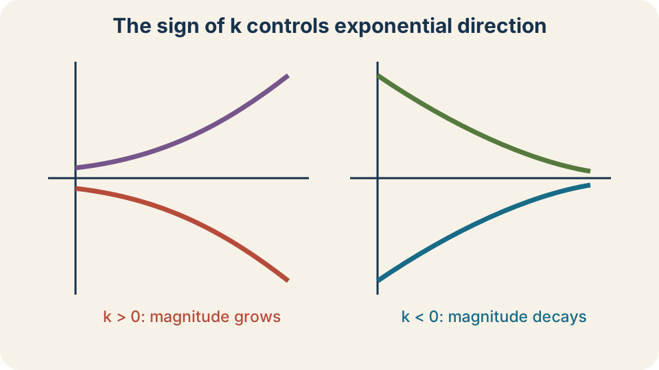
The sign of $k$ determines whether nonzero solutions grow or decay in magnitude. The equilibrium $y=0$ remains constant. Solution curves do not cross that equilibrium when uniqueness holds. The initial value sets the multiplicative constant. Reciprocal-time units in $k$ make the exponent dimensionless. Positive and negative branches retain their initial signs.

Apply an initial condition efficiently

An initial condition can be applied to an implicit relation before solving explicitly. Suppose integration gives $H(y)=G(t)+C$ and $y(t_0)=y_0$. Substitution yields $C=H(y_0)-G(t_0)$. The solution can then be written $H(y)-H(y_0)=G(t)-G(t_0)$. This definite-integral style often keeps constants and units organized.

One may instead use separated definite integrals: $\int_{y_0}^{y(t)}\frac{1}{h(u)}\,du=\int_{t_0}^{t}g(s)\,ds$. The letters $u$ and $s$ are dummy integration variables. Their bounds carry the initial and current states directly. Differentiating the left side uses the Fundamental Theorem and chain rule. This form avoids writing a free $C$ altogether.

Apply the condition only to a family valid on the relevant branch. If logarithms require $y>0$ or $y<0$, the initial sign selects the branch. If algebra produces multiple square-root branches, the initial value chooses one. An initial condition is more than a way to find a number. It identifies the trajectory and its interval of validity.

Solve a nonlinear power equation

Consider $y'=y^2$ with $y(0)=y_0$. First record the equilibrium $y=0$. For a nonzero branch, separation gives $y^{-2}\,dy=dt$. Integration produces $-\frac{1}{y}=t+C$. Solving gives $y=-\frac{1}{t+C}$.

Apply $y(0)=y_0\ne0$. The relation $-\frac{1}{y_0}=C$ yields $y(t)=\frac{y_0}{1-y_0t}$. Differentiation gives y'=rac{y_0^2}{(1-y_0t)^2}=y^2. The denominator cannot equal zero. Therefore the solution’s interval must avoid $t=\frac{1}{y_0}$.

If $y_0>0$, the solution grows and becomes unbounded at finite forward time $t=\frac{1}{y_0}$. If $y_0<0$, it increases toward zero for forward time while its singularity lies in the past. The equilibrium initial value $y_0=0$ yields $y(t)=0$, which division lost. Qualitative sign analysis predicts $y'\ge0$ for every state. The explicit solutions agree because they never decrease on their valid intervals.

Handle logarithms and absolute values

Integrals such as $\int\frac{1}{y-a}\,dy$ produce $\ln|y-a|+C$. The absolute value permits both branches $y>a$ and $y<a$. Exponentiating gives $|y-a|=Be^{G(t)}$ with $B>0$. A sign choice can be absorbed into a nonzero constant $A$. The result becomes $y-a=Ae^{G(t)}$.

Removing absolute values without accounting for sign can lose a solution branch. Writing $\ln(y-a)$ silently assumes $y>a$. That may be justified by an initial condition but must be stated. On intervals where a unique solution cannot cross equilibrium $y=a$, the initial side is preserved. The branch condition remains part of the solution.

Logarithm arguments should be dimensionless in physical models. More precisely, one can interpret $\ln\left|\frac{y-a}{y_{\mathrm{ref}}}\right|$ using a reference quantity with the same units. Constants introduced during integration absorb the reference scale in many classroom derivations. Unit awareness explains why subtracting logarithms to form a ratio is often natural. Formal symbols should remain compatible with physical dimensions.

Solve logistic growth while preserving equilibria

Consider $P'=rP\left(1-\frac{P}{K}\right)$, where $r>0$ has reciprocal-time units and $K>0$ has population units. Equilibria occur at $P=0$ and $P=K$. For non-equilibrium branches, $\frac{dP}{P(1-P/K)}=r\,dt$. Partial fractions decompose the state integrand. The result is $\ln|P|-\ln|K-P|=rt+C$ up to an absorbed constant factor.

Combining logarithms gives $\ln\left|\frac{P}{K-P}\right|=rt+C$. Exponentiating and solving yields $P(t)=\frac{K}{1+Ae^{-rt}}$. For initial value $P(0)=P_0$ with $0<P_0<K$, the constant is $A=\frac{K-P_0}{P_0}$. The solution stays between the two equilibria. It approaches $K$ as $t\to\infty$.

The phase line predicts this behavior before integration. For $0<P<K$, both factors on the right are positive, so population increases. For $P>K$, the factor $1-P/K$ is negative, so population decreases toward $K$. For negative mathematical states, the sign pattern can be analyzed even if the context excludes them. The formula should agree with those directional arrows.

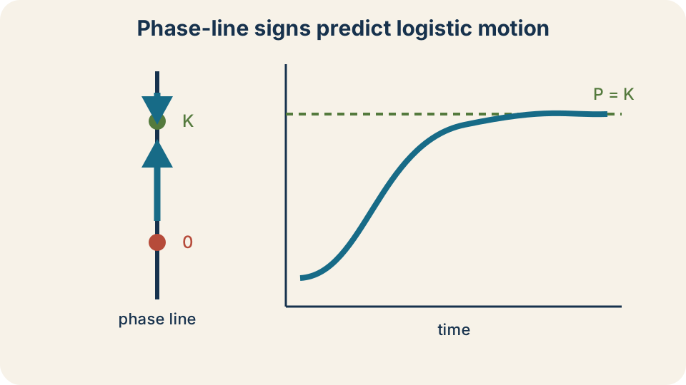
The equilibria are $P=0$ and $P=K$. Between them, the derivative is positive and solutions rise. Above $K$, the derivative is negative and solutions fall. The carrying capacity attracts positive nonzero states. The explicit logistic curve matches these phase-line directions. Initial position determines which branch is followed.

Model Newtonian cooling

Newton’s cooling model is $T'=-k(T-T_a)$, where $T_a$ is constant ambient temperature and $k>0$ has reciprocal-time units. The equilibrium is $T=T_a$. Define the temperature difference $u=T-T_a$. Since $T_a$ is constant, $u'=T'$. The equation becomes $u'=-ku$.

The proportional-decay solution gives $u(t)=u_0e^{-k(t-t_0)}$. Restoring temperature yields $T(t)=T_a+(T_0-T_a)e^{-k(t-t_0)}$. If $T_0>T_a$, the difference is positive and decays toward zero. If $T_0<T_a$, the difference is negative and its magnitude decays. In both cases temperature approaches ambient without crossing it under this ideal model.

Suppose $T_a=20.0\,{}^\circ\mathrm{C}$, $T_0=80.0\,{}^\circ\mathrm{C}$, $k=0.100\,\mathrm{min}^{-1}$, and $t_0=0\,\mathrm{min}$. After $10.0\,\mathrm{min}$, $T=20.0\,{}^\circ\mathrm{C}+(60.0\,{}^\circ\mathrm{C})e^{-1}\approx42.1\,{}^\circ\mathrm{C}$. The exponent is dimensionless because minutes cancel. The result lies between initial and ambient temperatures as qualitative reasoning requires. The positive temperature difference has decreased without changing sign.

Understand implicit solutions

Some separated integrals yield a relation that is difficult or impossible to isolate with elementary functions. An implicit relation $H(y)=G(t)+C$ can still define one or more solution branches. Differentiating it implicitly may recover the ODE. Numerical root finding can evaluate $y$ at chosen times. Explicit form is convenient but not the definition of a solution.

Even when explicit isolation is possible, implicit form may reveal structure more clearly. A logarithmic ratio can show equilibrium barriers and sign branches. A conserved combination may display invariant relationships. Premature exponentiation or squaring can introduce extraneous branches. Keep the clean implicit relation until the problem requires more.

When an implicit relation defines several local branches, the initial condition selects one through the implicit function theorem under appropriate derivative conditions. Points where the relevant derivative vanishes may require separate analysis. State intervals are important around singularities. A solution is a function on an interval, not merely a symbolic equation. Branch choice must remain consistent throughout that interval.

Determine the interval of validity

A differential-equation solution must be differentiable and satisfy the equation throughout its interval. Denominators in the explicit formula cannot vanish. Logarithm arguments must stay on a valid nonzero branch. The original differential equation may also be undefined at certain points. The maximal interval containing the initial time stops at the first obstruction.

For $y'=y^2$ with $y(0)=1$, the formula is $y=\frac{1}{1-t}$. It satisfies the equation for $t\ne1$. The maximal interval containing $0$ is $(-\infty,1)$. One cannot join across $t=1$ because the solution becomes unbounded. Writing only the formula without its interval is incomplete.

For exponential growth $y=y_0e^{kt}$, no finite denominator or logarithmic obstruction appears after the branch is resolved. The solution is defined for all real $t$ in the mathematical model. A physical context may still restrict time to $t\ge0$. Mathematical and contextual intervals should be distinguished. Both can matter when reporting an answer.

Verify with derivatives and initial data

Verification has three parts. First differentiate the proposed solution. Second substitute it into the original right-hand side and confirm equality. Third evaluate the initial time and confirm the initial state. A formula that satisfies the ODE but not the initial condition belongs to the wrong family member.

For $y=y_0e^{k(t-t_0)}$, differentiation gives $y'=ky_0e^{k(t-t_0)}=ky$. At $t=t_0$, the exponential is $1$, so $y(t_0)=y_0$. The formula is defined for all real time. These checks verify equation, data, and interval. They also confirm that the parameter $k$ appears with the correct sign.

For an implicit solution, differentiate both sides with respect to $t$. The chain rule introduces $y'$, which can be isolated and compared with the original ODE. Check any divisions made during recovery. Equilibrium branches should be verified separately. Verification is the final mathematical evidence, not an optional afterthought.

Use qualitative reasoning as an error check

Before integrating an autonomous equation $y'=h(y)$, mark the roots of $h$. Test the sign of $h$ between roots. Positive derivative means arrows upward on a phase line, and negative derivative means arrows downward. Stable equilibria attract nearby arrows, while unstable equilibria repel them. This picture predicts allowable motion.

A derived formula moving opposite the arrows contains a sign or algebra error. A formula crossing an equilibrium may violate uniqueness. A solution that grows when the right side is negative is immediately suspect. Limits of the formula should approach equilibria predicted by the phase line when appropriate. Qualitative analysis is a low-cost independent check.

Time-dependent factors $g(t)$ can reverse direction as time changes. In $y'=g(t)h(y)$, the sign is the product of both factors. A pure state phase line is most direct when $g$ has fixed sign or the equation is autonomous. Otherwise inspect time intervals separately. The same sign reasoning still applies locally.

Repair common mistakes

One mistake is dividing by $h(y)$ without first recording roots. This loses equilibrium solutions. Another is separating an equation whose right side cannot be factored into pure time and state pieces. Moving a mixed expression beside $dy$ does not make its integral a single-variable antiderivative. Classification must precede manipulation.

Another mistake is omitting absolute values after integrating $\frac{1}{y-a}$. This silently discards one sign branch. A related mistake is introducing $\pm$ without using the initial condition to select a branch. Constants can often absorb a fixed sign. Domain and interval statements clarify what the algebra means.

A final mistake is accepting a symbolic formula without verification. Division, exponentiation, squaring, and inversion can lose or add branches. Different constants that look different may describe the same family after reparameterization. Substitute into the original equation and initial condition. Then compare with units and qualitative behavior.

Retrieve and connect forward

For $y'=y^2$, the equilibrium initial condition is $y(0)=0$, producing $y(t)=0$. Dividing by $y^2$ assumes $y\ne0$ and removes that branch. For nonzero initial value $y_0$, the solution is $\frac{y_0}{1-y_0t}$ on the maximal interval containing zero. Positive initial values blow up in finite forward time. The phase-line sign $y'\ge0$ agrees with the formula.

For $y'=ky$, separation gives a logarithm and then an exponential family. The initial value fixes its multiplicative constant. For logistic growth, partial fractions expose two equilibrium factors and a carrying-capacity limit. For cooling, shifting by ambient temperature reduces the model to proportional decay. These examples reuse one structural method across different contexts.

Separable equations turn factorable local rates into integrated global relationships. The complete workflow is classify, record equilibria, separate on nonzero branches, integrate, apply data, determine intervals, and verify. Qualitative arrows and units strengthen the algebraic evidence. Equations that are not separable may require integrating factors, substitutions, or numerical methods. Recognizing method boundaries is part of solving differential equations well.