First-Order ODEs Model Growth, Decay, and Balance

A first-order ordinary differential equation relates an unknown function to its first derivative. It describes how a state changes rather than directly stating the state itself. That local rule can model growth, decay, heating, cooling, mixing, electrical response, and motion toward equilibrium. Different equation structures require different solution methods, but every trustworthy solution must satisfy the original equation and its data. This article builds a connected framework for interpretation, classification, exact methods, qualitative analysis, and numerical approximation.

Begin with a changing state and its rate

Let $y(t)$ represent a quantity that changes with independent variable $t$. The derivative $y'=dy/dt$ measures its instantaneous rate of change. A first-order equation contains $y'$ but no derivative of higher order. The adjective ordinary means there is one independent variable. The equation may still contain the variables $t$ and $y$ in complicated ways.

An explicit first-order equation is often written $y'=f(t,y)$. The function $f$ determines the rate at every allowed state-time pair. If $t$ is in seconds and $y$ is in kilograms, then $f$ must have units kilograms per second. This unit condition is not optional decoration. It checks whether the proposed mechanism could produce the stated change.

The equation does not usually specify one curve by itself. It describes a family of possible solution functions. Additional information, often $y(t_0)=y_0$, selects a member of that family. The pair $(t_0,y_0)$ is an initial condition. Together, the equation and initial condition form an initial-value problem.

Translate a mechanism into an equation

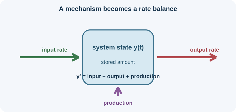
Modeling begins by identifying the state variable and the processes that increase or decrease it. A balance has the form rate of change equals input rate minus output rate plus internal production. Every term must share the units of the left side. Positive and negative signs come from the direction of transfer. A diagram of the system boundary often clarifies those signs.

For a population $P(t)$ with per-capita growth rate $r$, the simplest assumption is $P'=rP$. The parameter $r$ has units of inverse time so that $rP$ has units population per time. Positive $r$ models growth, while negative $r$ models decay. The assumption says each individual contributes equally and environmental limitations are ignored. Those assumptions define the model’s scope.

For a well-mixed tank, solute amount $A(t)$ changes by solute entering minus solute leaving. An inflow concentration multiplied by volumetric flow rate gives mass per time. The outflow concentration is often $A(t)/V(t)$ when mixing is uniform. Multiplying by outflow rate gives the second mass-per-time term. A correct differential equation emerges from the balance and units before any algebraic method is selected.

Read the equation through a slope field

For $y'=f(t,y)$, every point $(t,y)$ receives slope $f(t,y)$. Drawing short segments with those slopes creates a slope field. A solution curve must remain tangent to the field wherever it is differentiable. The field displays many possible initial conditions at once. It therefore reveals behavior before a formula is known.

Positive segments indicate locally increasing solutions. Negative segments indicate locally decreasing solutions. Horizontal segments occur where $f(t,y)=0$. Steepness indicates derivative magnitude, although displayed segment length is arbitrary. Axis scaling must be considered when reading numerical slopes from angles.

An initial point selects one path through the field. Under suitable existence and uniqueness conditions, one local solution passes through that point. Distinct solutions then cannot cross at an ordinary point because crossing would assign two paths to one initial condition. A coarse sketch can falsely appear to cross. The theorem, not graphical neatness, supports the noncrossing claim.

Classify structure before choosing a method

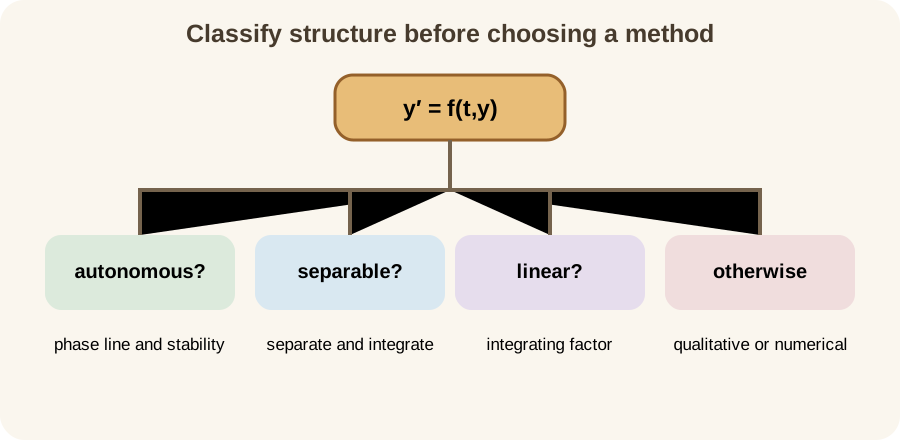
Method selection begins by rewriting the equation clearly. Ask whether it is autonomous, separable, linear, exact, or recognizable through substitution. More than one classification may apply. The equation $y'=1-y$ is autonomous, separable, and linear. Different methods can therefore solve it and check one another.

An autonomous equation has form $y'=f(y)$ with no explicit independent variable. A separable equation can be written $y'=g(t)h(y)$. A linear equation can be written $y'+p(t)y=q(t)$. These labels describe algebraic structure rather than the physical application. A cooling law and electrical circuit can share the same mathematical form.

Classification also considers the requested output. A stability question may need only a sign chart. A numerical trajectory may not require a closed-form solution. A precise parameter formula may justify symbolic work. Choosing the simplest method that answers the actual question reduces unnecessary manipulation.

Solve separable equations without losing equilibria

A separable equation has form $dy/dt=g(t)h(y)$. Where $h(y)\neq0$, rearrange to $\dfrac{1}{h(y)}\,dy=g(t)\,dt$. Integrating gives $\int\dfrac{1}{h(y)}\,dy=\int g(t)\,dt+C$. The constant $C$ represents one combined integration constant. The resulting relation may be implicit or explicitly solvable for $y$.

Division by $h(y)$ can discard solutions for which $h(y)=0$. Find those constant equilibrium solutions before dividing. For logistic growth $P'=rP(1-P/K)$, equilibria are $P=0$ and $P=K$. Separation treats non-equilibrium solutions. The complete solution set must include the constant cases separately.

After integrating, apply the initial condition while the algebra remains stable. Absolute values from logarithmic antiderivatives should not be dropped without justification. Exponentiating may convert an additive constant into a nonzero multiplicative constant. Domain restrictions can split solution families. Substitution into the original equation verifies that algebraic transformations did not introduce or lose behavior.

Derive exponential growth and decay

For $y'=ky$, separation gives $dy/y=k\,dt$ when $y\neq0$. Integration yields $\ln|y|=kt+C$. Exponentiating gives $|y|=e^Ce^{kt}$. Absorbing sign and the positive factor $e^C$ into one constant produces $y=Ce^{kt}$. The equilibrium $y=0$ is included when $C=0$.

Applying $y(0)=y_0$ gives $C=y_0$. Therefore $y(t)=y_0e^{kt}$. If $k>0$, magnitude grows exponentially. If $k<0$, it decays toward zero. The parameter $k$ must have units inverse time because the exponent $kt$ must be dimensionless.

Doubling time for positive $k$ satisfies $e^{kT_2}=2$, so $T_2=\dfrac{\ln2}{k}$. Half-life for negative $k$ satisfies $e^{kT_{1/2}}=\dfrac12$, giving $T_{1/2}=\dfrac{\ln2}{|k|}$. Both times inherit units from $1/k$. These formulas connect a differential rate parameter to observable time scales. Substituting either time into the exponential solution verifies its intended factor change.

Solve linear equations with an integrating factor

A first-order linear equation in standard form is $y'+p(t)y=q(t)$. The coefficient of $y'$ must be one before the method is applied. The function $p(t)$ multiplies the unknown state. The function $q(t)$ acts as a forcing or input. Neither coefficient may depend nonlinearly on $y$ in a linear equation.

Define the integrating factor $\mu(t)=e^{\int p(t)\,dt}$. Multiplying the standard equation by $\mu$ gives $\mu y'+\mu p y=\mu q$. Because $\mu'=p\mu$, the left side equals the product derivative $(\mu y)'$. Integration then gives $\mu y=\int\mu q\,dt+C$. Finally, divide by $\mu$ to recover $y$.

The integrating factor is engineered, not guessed magically. It makes the product rule appear on the left. Multiplying by a nonzero factor preserves equation equivalence. One can verify the result by differentiating $\mu y$. Understanding this construction reduces memorization and helps detect a sign error in the exponent.

Work a forced linear example

Consider $y'+2y=6$ with $y(0)=1$. Here $p(t)=2$ and $q(t)=6$. The integrating factor is $\mu=e^{2t}$. Multiplying gives $e^{2t}y'+2e^{2t}y=6e^{2t}$. The left side is $(e^{2t}y)'$.

Integration yields $e^{2t}y=3e^{2t}+C$. Dividing by $e^{2t}$ gives $y=3+Ce^{-2t}$. Applying $y(0)=1$ gives $C=-2$. Thus the solution is $y(t)=3-2e^{-2t}$. Direct substitution confirms $y'+2y=6$.

The constant level $y=3$ is the equilibrium because $0+2(3)=6$. The transient term $-2e^{-2t}$ decays toward zero. The solution therefore approaches three from below. This long-term behavior is visible in the equation before solution because rates are positive below three and negative above three. Algebra and qualitative analysis tell the same story.

Analyze autonomous equilibria and stability

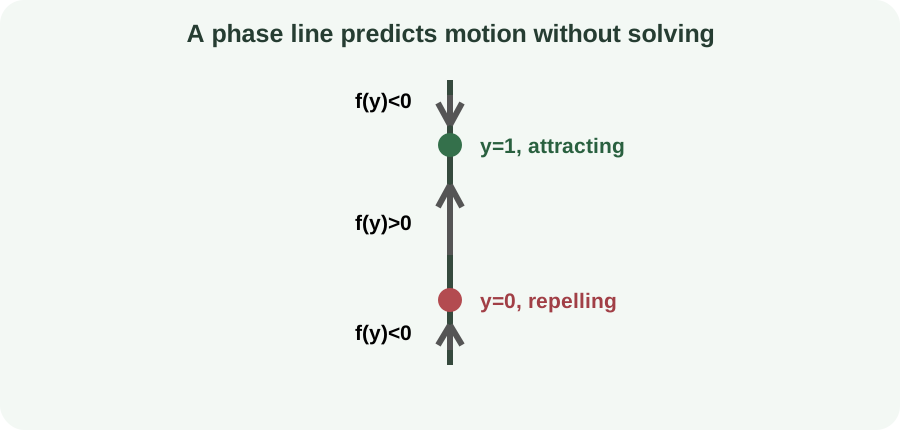
For autonomous equation $y'=f(y)$, equilibria satisfy $f(y_*)=0$. The subscript star labels a constant state. A phase line places equilibria on a one-dimensional axis and marks the sign of $f$ between them. Positive sign arrows point toward increasing $y$. Negative sign arrows point toward decreasing $y$.

An equilibrium is attracting when nearby arrows point toward it from both sides. It is repelling when arrows point away on both sides. It is semistable when one side approaches and the other departs. These terms describe local dynamics. Global behavior may involve other equilibria, domain boundaries, or unbounded growth.

For $y'=y(1-y)$, equilibria are zero and one. Between zero and one, the derivative is positive. Above one, it is negative, so trajectories move back toward one. Below zero, it is negative, so trajectories move farther downward. Therefore one is attracting and zero is repelling.

Model approach to environmental equilibrium

Newton’s cooling law is $T'=-k(T-T_{\mathrm{env}})$, where $k>0$. Temperature $T$ and environmental temperature $T_{\mathrm{env}}$ share units, such as degrees Celsius. Their difference is a temperature difference. Therefore $k$ has units inverse time. The negative sign drives temperature toward the environment.

If $T>T_{\mathrm{env}}$, the difference is positive and $T'<0$, so the object cools. If $T<T_{\mathrm{env}}$, the difference is negative and $T'>0$, so it warms. At equality, $T'=0$. The environment temperature is therefore an attracting equilibrium. This sign reasoning does not require explicit solution.

For constant environment, the solution is $T(t)=T_{\mathrm{env}}+(T_0-T_{\mathrm{env}})e^{-kt}$. The initial temperature is $T_0$. The exponential factor is dimensionless and decays toward zero. The temperature difference therefore shrinks exponentially. Real cooling may depart from the model when radiation, phase changes, or varying environments matter.

Approximate solutions with Euler’s method

Not every first-order equation has a convenient elementary solution. Euler’s method approximates $y'=f(t,y)$ from initial pair $(t_n,y_n)$. With step $h$, the update is $y_{n+1}=y_n+h f(t_n,y_n)$. The method follows the current tangent line for one step. It then reevaluates the slope at the new point.

The product $h f(t_n,y_n)$ has units of $y$. If $h$ is in seconds and $f$ in metres per second, their product is metres. This dimensional check supports the update formula. Smaller steps usually reduce local error. They also require more computation and do not automatically cure every stability problem.

For $y'=1-y$, $y(0)=2$, and $h=0.100\,\mathrm s$, suppose $y$ is dimensionless and the rate unit is inverse seconds. The first slope is $-1.00\,\mathrm{s^{-1}}$. The update gives $y_1=2.00+(0.100\,\mathrm s)(-1.00\,\mathrm{s^{-1}})=1.90$. Repeating produces a numerical path toward equilibrium one. Comparing this step with the exact solution provides a local accuracy check.

Distinguish exact, implicit, and numerical answers

An explicit solution writes $y$ directly as a function of the independent variable. An implicit solution relates $t$ and $y$ without isolating $y$. Both can be exact. A numerical solution provides approximate values at selected points. The appropriate representation depends on the equation and the question.

Implicit relations may contain multiple branches. An initial condition selects the relevant branch and domain. Solving algebraically for $y$ can introduce square roots or other branch choices. Numerical methods may cross boundaries if steps are too large. Every representation requires attention to domain and uniqueness.

Exact does not mean physically perfect. A formula can solve an idealized model exactly while the model only approximates reality. Numerical does not mean conceptually inferior. Many important models require computation. Accuracy claims should distinguish equation-solving error from model-form error and parameter uncertainty.

Verify a proposed solution completely

Verification begins by differentiating the proposed function. Substitute both the function and derivative into the original equation. Simplify the two sides until equality is visible. Then check the initial or boundary data separately. A solution that satisfies only the equation may belong to the wrong family member.

Units and domains form additional checks. A logarithm or exponential must receive a dimensionless argument. Denominators must remain nonzero on the claimed interval. Square roots require appropriate signs. A formula valid locally may fail beyond a singular time.

Qualitative behavior provides another independent check. If the phase line predicts an attracting equilibrium, a proposed solution that races away is suspicious. If the slope field is positive in a region, a solution cannot decrease there. If a nonnegative population model produces negative values, inspect domain or numerical error. Agreement among substitution, data, units, and geometry builds confidence.

Diagnose recurring method errors

One error is separating a nonseparable equation by moving additive terms as though they were factors. Another is dividing by a state factor without recording its zero equilibria. A third is applying an integrating factor before standardizing the coefficient of $y'$. A fourth is forgetting the arbitrary integration constant. Classification and a written checklist prevent these mistakes.

Sign errors often corrupt physical interpretation. Define the positive direction for transfers. Test the model above and below an expected equilibrium. A restoring law should point toward equilibrium on both sides. If it does not, either the sign or the mechanism needs reconsideration.

Numerical output can appear smooth while being wrong. Compare two step sizes and inspect whether results converge. Plot the numerical points against a slope field. Monitor invariant signs, bounds, or conserved quantities when available. A computer evaluates instructions faithfully, so validation remains the modeler’s responsibility.

Practice classification and solution strategy

Classify $y'=t+y$. It is not autonomous because $t$ appears explicitly. It is not separable into one factor of $t$ times one factor of $y$. Rewriting as $y'-y=t$ shows that it is linear. An integrating factor is therefore a natural exact method.

Classify $y'=ty(1-y)$. It is separable because the right side is a product of $t$ and a function of $y$. It is not autonomous because $t$ appears explicitly. Equilibria $y=0$ and $y=1$ must be saved before division. A slope field can still reveal time-dependent changes in steepness.

For each equation, state what the desired answer requires. If only long-term stability is asked, begin qualitatively. If a parameter must be inferred from data, derive a usable formula. If no convenient exact family applies, choose a numerical method with an error check. Structure and purpose should determine the workflow.

Connect the foundational methods

Slope fields convert a derivative rule into geometry. Phase lines compress autonomous behavior into sign information. Separation exploits multiplicative structure. Integrating factors exploit linear product-rule structure. Numerical methods follow local slopes when symbolic tools are unavailable or unnecessary.

These approaches are complementary rather than competitors. A field predicts behavior, an exact solution supplies precision, and numerical results handle broader models. Units and substitution validate all three. Comparing representations often exposes an error that one method alone would conceal. Mature differential-equation work moves among them deliberately.

You are ready to continue when you can identify the state, rate, units, and initial data in a model. You should classify structure before manipulating the equation. You should preserve equilibria, derive integrating factors, interpret stability, and validate numerical steps. These habits make first-order ODEs a coherent modeling language rather than a list of tricks. Specialized lessons can now deepen each method without losing the larger map.