Slope Fields Show an ODE Before It Is Solved

A first-order differential equation specifies local change before it provides a formula for a solution. A slope field turns that local rule into a picture made from short line segments. Each segment reports the derivative that a solution would have if it passed through that point. Curves that remain tangent to the segments represent possible solutions. This geometric view reveals entire families of behavior before symbolic or numerical solution methods are applied.

Read an equation as a direction rule

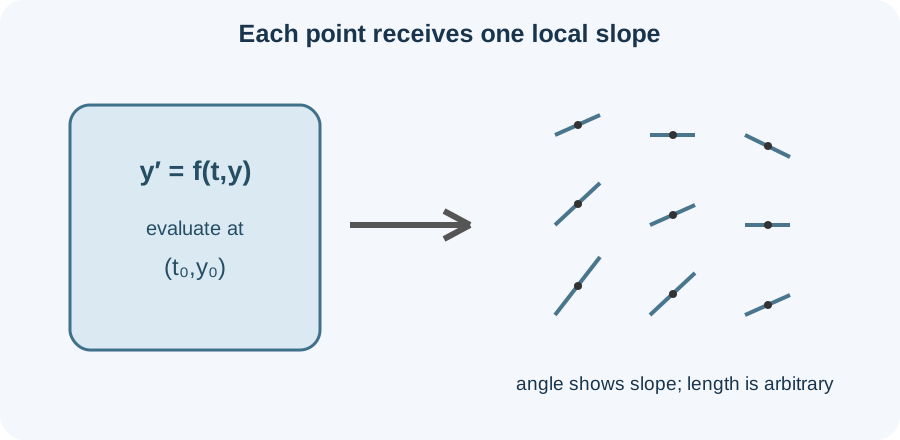
An explicit first-order ordinary differential equation has the form $y'=f(t,y)$. The prime means $dy/dt$, the instantaneous rate of change of $y$ with respect to $t$. The function $f$ assigns a numerical slope to every point $(t,y)$ in its domain. The independent variable is placed on the horizontal axis, and the dependent variable is placed on the vertical axis. A slope field samples this assignment at a finite grid of points.

At grid point $(t_0,y_0)$, evaluate $m=f(t_0,y_0)$. Draw a short segment centered at that point with rise-to-run ratio $m$. A positive value tilts upward from left to right. A negative value tilts downward, while zero produces a horizontal segment. Segment length is chosen for legibility and carries no mathematical meaning.

The field is not a collection of little solution curves. Each segment records only local tangent information at one point. A genuine solution must pass through continuously while matching the prescribed slope everywhere. The field therefore acts like a landscape of permitted directions. It constrains motion without yet selecting one path.

Connect derivative meaning to segment angle

The derivative is a rate measured in units of $y$ per unit of $t$. If $t$ is measured in seconds and $y$ in metres, then $y'$ has units of metres per second. A displayed angle depends on the relative axis scales. Stretching one axis visually changes segment angles even though numerical slopes remain unchanged. Meaning belongs to the coordinate ratio, not to an uncalibrated visual impression.

A segment with slope $2$ represents about two vertical units gained for one horizontal unit. A segment with slope $-\dfrac{1}{2}$ represents one vertical unit lost for every two horizontal units. A vertical segment would correspond to unbounded slope and usually does not arise from an explicit finite function $f(t,y)$. Steep segments indicate large derivative magnitude. Shallow segments indicate slower local change.

Axis labels and scale marks are therefore part of the mathematics. A field without them can still suggest qualitative patterns, but it cannot support precise numerical reading. Computer graphics often normalize segment lengths so steep pieces do not dominate the picture. That normalization leaves orientation intact. Readers should inspect angle and location rather than comparing drawn lengths.

Construct a field systematically

Begin by selecting a rectangular viewing window and grid spacing. Evaluate $f(t,y)$ at every grid point. Convert each resulting slope into a short centered segment. Use one consistent displayed length so density remains readable. Label axes, units, the differential equation, and any important nullclines.

For $y'=t-y$, the point $(0,2)$ has slope $-2$. The point $(1,1)$ has slope $0$. The point $(2,0)$ has slope $2$. These samples already show a transition from downward to horizontal to upward tilt. A larger grid reveals where that transition occurs throughout the plane.

Hand construction becomes efficient when structure is used before arithmetic. Look for curves on which the slope has one constant value. Use symmetry, repeated rows, or repeated columns when the formula allows them. Calculate representative points to verify the pattern. Randomly filling isolated segments is slower and more error-prone than mapping the equation’s organization.

Use isoclines to organize repeated slopes

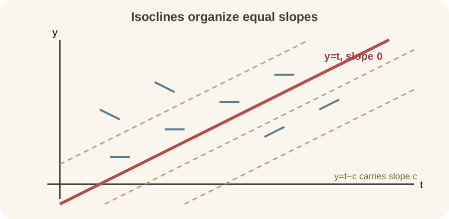
An isocline is a curve along which $f(t,y)$ equals a constant $c$. Every field segment on that curve has slope $c$. The equation $f(t,y)=0$ defines a zero isocline, often called a nullcline. Segments on it are horizontal. Isoclines provide a scaffold for the full field.

For $y'=t-y$, the isocline with slope $c$ satisfies $t-y=c$, or $y=t-c$. The zero-slope isocline is $y=t$. Below this line, $t-y$ is positive and segments tilt upward. Above it, $t-y$ is negative and segments tilt downward. Parallel lines $y=t-c$ carry every other fixed slope.

An isocline is generally not a solution curve. A curve can carry horizontal field segments without itself being horizontal. For $y'=t-y$, the line $y=t$ has slope one as a geometric line, but the differential equation prescribes slope zero at its points. Therefore a solution crossing that line has a horizontal tangent rather than following it. Comparing curve slope with prescribed field slope prevents this common confusion.

Sketch a solution through an initial condition

An initial condition $y(t_0)=y_0$ selects a point through which the desired solution must pass. Begin at $(t_0,y_0)$ and follow the nearby segment direction. As the curve moves, continuously adjust its tangent to match neighboring segments. Sketch both forward and backward in $t$ when the domain allows. A smooth curve should flow through the field rather than connect segment endpoints like a polygon.

For $y'=t-y$ with $y(0)=2$, the initial slope is $-2$. The curve initially decreases. As it approaches the zero-slope line $y=t$, its downward slope becomes less negative. At a crossing, the curve has a horizontal tangent. Afterward the surrounding field determines whether the curve rises or returns.

The sketch is qualitative, not an exact graph. It should capture monotonicity, turning behavior, equilibrium approach, and relative steepness. A slope field cannot provide many accurate decimal places by eye. Its strength is global organization across many initial conditions. Numerical or analytic methods can later refine one selected trajectory.

Recognize autonomous equations and equilibria

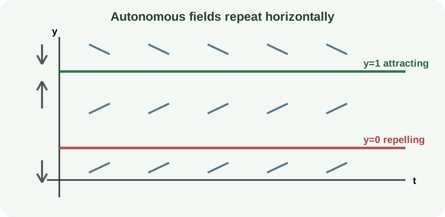
An autonomous equation has the form $y'=f(y)$ with no explicit $t$ dependence. Every point at the same height has the same slope. The field therefore repeats horizontally in rows. This visible repetition is a diagnostic feature. Horizontal translation of a solution produces another solution when the equation is autonomous.

An equilibrium solution is a constant function $y(t)=y_*$ satisfying $f(y_*)=0$. The star labels an equilibrium value and does not mean multiplication. Every segment along horizontal line $y=y_*$ is horizontal. A solution starting exactly there remains there. Equilibria divide the plane into horizontal bands with consistent sign patterns.

For $y'=y(1-y)$, equilibria occur at $y=0$ and $y=1$. Between them, both factors are positive, so solutions increase. Above one, the factor $1-y$ is negative, so solutions decrease. Below zero, $y$ is negative while $1-y$ is positive, so solutions also decrease. This sign analysis predicts behavior without solving the logistic equation.

Classify attraction and repulsion

An equilibrium is locally attracting when nearby solution arrows point toward it from both sides. It is locally repelling when nearby arrows point away on both sides. A semistable equilibrium attracts from one side and repels from the other. These classifications concern neighboring trajectories. They do not require a closed-form solution.

For $y'=y(1-y)$, solutions just below $1$ increase while those just above $1$ decrease. Both directions point toward $y=1$, so it is attracting. Near $y=0$, values just above zero increase and those just below zero decrease. Both directions point away from zero, so it is repelling. The field turns a sign chart into visible long-term dynamics.

Attraction does not guarantee that every initial condition approaches the equilibrium. The classification may be local, and other equilibria or singularities can organize distant behavior. Domain restrictions also matter. A complete statement names the interval of initial values being considered. Qualitative conclusions should match the region actually displayed and analyzed.

Predict increasing, decreasing, and turning behavior

Where $f(t,y)>0$, solution curves increase as $t$ increases. Where $f(t,y)<0$, they decrease. Where $f(t,y)=0$, a solution passing through has a horizontal tangent. These are local statements. The curve’s next behavior depends on which sign region it enters.

A horizontal tangent need not be a local maximum or minimum. If a solution crosses a zero isocline from a negative-slope region into a positive-slope region, it has a local minimum. Reversing that sign change produces a local maximum. Touching a nullcline without changing sign can create a stationary inflection-like event. Inspect both sides rather than labeling every flat tangent as a turning point.

Concavity can also be inferred by watching how prescribed slopes change along a solution. If slopes become more positive as the curve advances, the solution tends to be concave upward. If they become more negative, it tends to be concave downward. Formally, differentiating gives $y''=f_t+f_y y'$. The subscripts denote partial derivatives of the direction function.

Understand existence, uniqueness, and crossing

A slope field visually suggests that one permitted direction passes through each point. That fact alone does not guarantee one unique solution. A standard theorem gives local existence and uniqueness when $f$ and an appropriate derivative such as $f_y$ are continuous near the initial point. These are sufficient conditions. The theorem converts regularity of the slope rule into predictability of the initial-value problem.

When uniqueness holds, two distinct solutions cannot cross at the same point. A crossing would give the same initial condition two different future or past paths. This would contradict uniqueness. The statement applies within a region where theorem conditions hold. Curves may appear to cross in a coarse drawing because of sketching error.

Nonuniqueness can occur when the slope rule lacks sufficient regularity. The equation $y'=3y^{2/3}$ near $y=0$ admits behavior that can remain at equilibrium for a time and then depart. A slope field may not make this subtlety obvious at ordinary resolution. Therefore a picture supports intuition but does not replace theorem hypotheses. Qualitative reading and analytic justification should work together.

Compare slope fields with solution formulas

An explicit formula can answer precise questions for a particular family of solutions. A slope field shows many initial conditions simultaneously. It can reveal stable levels, barriers, and rapid-growth regions even when integration is difficult. These methods answer different questions. One should be used to check the other whenever both are available.

For $y'=t-y$, rewriting gives $y'+y=t$. Solving the linear equation yields $y=t-1+Ce^{-t}$. The constant $C$ identifies the member of the solution family. For $y(0)=2$, substitution gives $C=3$. The resulting curve initially has slope $-2$ and eventually approaches the line $y=t-1$, matching the field prediction.

Substituting an analytic solution back into the differential equation is essential. Differentiate the proposed formula and compare it with $f(t,y(t))$. Check the initial condition separately. Then compare its shape with the field’s signs and isoclines. Agreement across algebraic and graphical representations is stronger evidence than either alone.

Connect slope fields to Euler’s method

Euler’s method turns local slope information into a numerical stepping rule. Starting from $(t_n,y_n)$ with step size $h$, it uses $y_{n+1}=y_n+h f(t_n,y_n)$. The increment $h$ changes the independent variable. The product $h f(t_n,y_n)$ predicts the corresponding vertical change. Each step follows the tangent line for a short distance.

On a slope field, Euler’s method appears as a chain of small straight moves aligned with sampled segments. A smaller step usually tracks curvature more closely. Error accumulates because the slope changes continuously while each Euler step holds it fixed. The field makes this geometric source of error visible. Numerical approximation is therefore a disciplined version of tangent-following.

For $y'=t-y$, $y(0)=2$, and $h=0.1$, the first update is $y_1=2+0.1(0-2)=1.8$. Units are consistent when $h$ has units of $t$ and $f$ has units of $y$ per $t$. Their product has units of $y$. The next step reevaluates the slope at $(0.1,1.8)$. Repeated reevaluation lets the polygonal path adapt to the field.

Diagnose misleading pictures and common errors

One error is treating segment length as derivative magnitude. Many plotting systems normalize all segments for readability. Another is drawing a curve that follows the endpoints of little segments rather than remaining tangent. A third is confusing a nullcline with a solution. Reading what each graphical object represents prevents these mistakes.

Window choice can hide important behavior. A narrow vertical range may omit an equilibrium. A coarse grid may conceal rapid slope changes or singularities. Unequal axis scales can distort apparent angles. A responsible plot states its window and samples more densely where the direction rule varies rapidly.

The field also has a domain. If $f(t,y)$ is undefined on a curve, no segments should be drawn there. Solutions may stop, approach, or be unable to cross such a boundary. Filling undefined locations with horizontal or vertical marks invents information. Domain analysis must occur before qualitative interpretation.

Practice a complete qualitative analysis

For $y'=y(1-y)$, first locate all equilibria. Build a sign chart for the intervals below zero, between zero and one, and above one. Translate those signs into repeated horizontal rows of slopes. Classify each equilibrium as attracting or repelling. Then sketch solutions from one initial point in each interval.

For $y'=t-y$, derive isoclines $y=t-c$ for several values of $c$. Mark the zero-slope line and shade regions of positive and negative derivative. Sketch the solution through $(0,2)$ without using the exact formula. Identify where a horizontal tangent may occur. Compare the sketch with $y=t-1+3e^{-t}$ afterward.

Finally, create a field for $y'=t^2-y^2$. Locate zero isoclines by solving $t^2-y^2=0$. Explain why the two lines $y=t$ and $y=-t$ organize sign changes. Choose an initial point and predict whether the solution initially rises or falls. Use a few Euler steps to test the prediction numerically.

Carry qualitative reasoning forward

Slope fields introduce the central differential-equation habit of studying behavior before seeking formulas. Phase lines compress autonomous one-dimensional fields into sign diagrams. Phase planes extend the idea to systems with two dependent variables. Nullclines, equilibria, and stability remain central in those settings. The visual vocabulary learned here scales beyond scalar equations.

Numerical solvers also rely on repeated local derivative information. More advanced methods improve on Euler’s single slope by sampling several slopes within each step. Error control adjusts step size when the field changes rapidly. A qualitative field helps users recognize when a numerical path behaves implausibly. Computation becomes safer when paired with prior structural expectations.

You are ready to continue when you can translate $y'=f(t,y)$ into segment directions and explain what the segment length does not mean. You should identify isoclines, equilibria, sign regions, and likely solution behavior. You should state the assumptions behind noncrossing and uniqueness claims. These abilities let a differential equation communicate before it is explicitly solved. Analytic and numerical methods can then refine a picture that already makes conceptual sense.