Euler’s Method Follows an ODE One Step at a Time

A differential equation can describe a solution through its local slope even when no convenient formula for the whole solution is available. Euler’s method turns that slope information into a sequence of approximate points. At each point, it follows the current tangent line for a short step, then recomputes the slope. Repetition produces a numerical trajectory. The method is simple enough to calculate by hand and rich enough to expose the central ideas of numerical simulation.

Simplicity does not make the method automatically trustworthy. Step size controls truncation error, computational work, and sometimes numerical stability. A table printed to many decimal places can still be far from the true solution. A responsible computation therefore includes units, a refinement study, and a check against qualitative behavior. This article develops that reasoning from the initial-value problem through stability analysis.

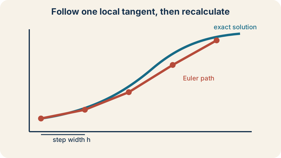
Euler’s method begins at a known initial point. It uses the differential equation to find the local tangent slope. A finite step along that tangent predicts the next point. The slope is then recalculated at the predicted point. Curvature creates a gap between the tangent step and the true solution.

State the initial-value problem

Consider the first-order initial-value problem $y'=f(t,y)$ with $y(t_0)=y_0$. The prime denotes derivative with respect to $t$, so $y'=\frac{dy}{dt}$. The function $f$ supplies the slope at any state point $(t,y)$. The initial condition gives one known point $(t_0,y_0)$ on the desired solution. Together, the rule and point determine the trajectory under appropriate existence and uniqueness conditions.

The independent variable $t$ often represents time, but it can represent any ordered input. The dependent variable $y(t)$ is the evolving state. If $y$ is measured in metres and $t$ in seconds, then $f$ has units $\frac{\mathrm{m}}{\mathrm{s}}$. Those slope units become important when the method multiplies by a time step. Dimensional consistency ensures that a state increment can be added to the previous state.

Euler’s method creates grid points $t_n=t_0+nh$, where $n$ is a nonnegative integer and $h$ is the step size. The approximation at $t_n$ is written $y_n$. In general, $y_n$ is not exactly equal to $y(t_n)$. The subscript labels a numerical sequence rather than a derivative. Keeping approximate and exact notation distinct prevents circular reasoning about error.

Derive the Euler update

The derivative definition gives $y'(t_n)\approx\frac{y(t_n+h)-y(t_n)}{h}$ for small nonzero $h$. Solving this approximation for the future value gives $y(t_n+h)\approx y(t_n)+hy'(t_n)$. The differential equation replaces $y'(t_n)$ with $f(t_n,y(t_n))$. Replacing exact states with numerical approximations produces $y_{n+1}=y_n+hf(t_n,y_n)$. The time update is $t_{n+1}=t_n+h$.

The product $hf(t_n,y_n)$ is the predicted change in $y$. If $h$ has seconds and $f$ has metres per second, the product has metres. Adding it to $y_n$ is therefore dimensionally valid. A positive product increases the next state, while a negative product decreases it. The method follows the sign and magnitude of the current local slope.

Geometrically, the formula evaluates the tangent line at a horizontal displacement $h$. The tangent line through $(t_n,y_n)$ is $L(t)=y_n+f(t_n,y_n)(t-t_n)$. Substituting $t=t_n+h$ gives the Euler update. The method then discards that line and constructs a new tangent at the next approximate point. It is a piecewise-tangent model of the solution.

Organize computation in a table

A reliable Euler table includes columns for $n$, $t_n$, $y_n$, slope $f(t_n,y_n)$, increment $h f(t_n,y_n)$, and next value $y_{n+1}$. Separating slope from increment reduces substitution errors. It also keeps units visible. The next row begins with the previous row’s output. Each step should use the current pair rather than an outdated initial value.

Suppose $y'=t+y$, $y(0)=1$, and $h=0.100\,\mathrm{s}$. At $(t_0,y_0)=(0\,\mathrm{s},1)$, the slope is $f(0,1)=1\,\mathrm{s}^{-1}$ if $y$ is dimensionless. The increment is $(0.100\,\mathrm{s})(1\,\mathrm{s}^{-1})=0.100$. Therefore $t_1=0.100\,\mathrm{s}$ and $y_1=1.100$. The reciprocal-second factor cancels the second in the step.

At the new point, the slope is $f(0.100,1.100)=1.200\,\mathrm{s}^{-1}$. The next increment is $0.120$, giving $y_2=1.220$ at $t_2=0.200\,\mathrm{s}$. Reusing the original slope would incorrectly turn Euler’s method into one long fixed tangent. Recalculation is what allows the polygonal path to bend. A table makes that repeated logic auditable.

Work the exponential-growth recurrence

Approximate $y'=y$, $y(0)=1$, on $0\le t\le1$ with $h=0.250$. The slope rule is $f(t,y)=y$. Euler’s update becomes $y_{n+1}=y_n+0.250y_n=1.250y_n$. Each step multiplies the current approximation by $1.250$. Four steps reach $t=1$.

The values are $y_0=1.000$, $y_1=1.250$, $y_2=1.5625$, $y_3=1.953125$, and $y_4=2.44140625$. The exact solution is $y(t)=e^t$, so $y(1)=e\approx2.71828$. The Euler value underestimates by about $0.27687$. Relative error is approximately $\frac{0.27687}{2.71828}\times100\%=10.2\%$. Printed digits beyond justified accuracy do not repair that discrepancy.

The underestimation can be predicted geometrically. The exponential solution is increasing and concave up. Its tangent line lies below the curve immediately to the right of each contact point. Euler repeatedly steps along those lower tangent lines. The sign of error is therefore connected to curvature, not accidental arithmetic.

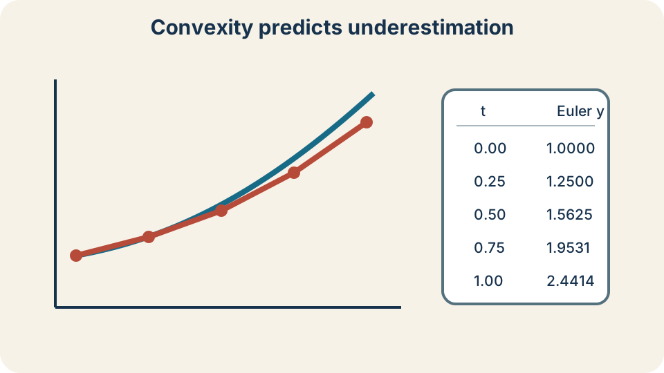
For $y'=y$, each Euler slope equals the current approximate height. A step of $0.250$ multiplies that height by $1.250$. The exact exponential curve bends upward above each forward tangent segment. Euler therefore underestimates in this example. Smaller steps shorten the interval over which each tangent is trusted. The geometric prediction agrees with the computed values.

Explain local truncation error

Taylor’s formula gives $y(t_n+h)=y(t_n)+hy'(t_n)+\frac{h^2}{2}y''(\xi_n)$ for some point $\xi_n$ between $t_n$ and $t_n+h$ under suitable smoothness. Euler’s step keeps the first two terms and omits the curvature term. Starting from the exact state, the omitted amount is proportional to $h^2$. This one-step discrepancy is called local truncation error. Its coefficient depends on the second derivative along the solution.

The phrase “proportional to $h^2$” means halving $h$ reduces a typical local error by roughly a factor of four when the asymptotic regime is reached. It does not mean every problem has the same error constant. Large curvature can make even a small step inaccurate. A nonsmooth solution can invalidate the simple estimate. Error order describes scaling under stated regularity conditions.

Local truncation error is not the same as floating-point roundoff. Truncation comes from replacing a curved solution by a tangent line over finite width. Roundoff comes from representing numbers with finite digits. Reducing $h$ usually reduces truncation error, while an extremely large number of steps can accumulate roundoff and cost. Numerical design balances these effects rather than assuming smaller is infinitely better.

Explain accumulated global error

Over a fixed interval, reducing $h$ increases the number of steps roughly like $\frac{1}{h}$. Each step introduces local error of order $h^2$, and previous errors also influence later slope evaluations. Under standard smoothness and stability assumptions, Euler’s global error is order $h$. This means halving the step typically halves the final error. Euler’s method is therefore called a first-order method.

The simple multiplication $\frac{1}{h}\cdot h^2=h$ offers intuition, but a full proof must control error propagation. If nearby trajectories separate rapidly, earlier errors can be amplified. Lipschitz conditions on $f$ help bound that amplification. The final constant can grow with interval length and problem sensitivity. Order alone does not give a guaranteed numerical value.

Global error compares $y_n$ with the exact $y(t_n)$ after many steps. It differs from the change between two approximate step sizes. Step refinement provides evidence about error but not an exact answer by itself. When the expected first-order regime holds, the difference between $h$ and $\frac{h}{2}$ solutions is comparable to the finer solution’s remaining error. This makes step halving a practical diagnostic.

Use step halving as evidence

For $y'=y$, $y(0)=1$, Euler with $h=0.500$ gives $y(1)=1.5^2=2.25$. With $h=0.250$, it gives $1.25^4\approx2.4414$. With $h=0.125$, it gives $1.125^8\approx2.5658$. The values move toward $e\approx2.7183$. Successive changes shrink, which supports convergence.

The errors are approximately $0.4683$, $0.2769$, and $0.1525$. Halving the step does not exactly halve these coarse-grid errors, but the ratio trends toward first-order behavior. Continuing refinement would move into the asymptotic regime more clearly. A table of step size, approximation, and change communicates more than one isolated output. Convergence evidence should accompany a reported numerical result.

If successive refinements do not stabilize, several explanations are possible. The step may still be too large, the problem may be stiff, the method may be unstable, or implementation may be wrong. A smaller difference does not prove proximity to the exact solution in every pathological case. Compare qualitative behavior and, when possible, use a higher-order reference method. Numerical confidence comes from converging lines of evidence.

Distinguish accuracy from stability

Accuracy asks how close the approximation is to the exact solution. Stability asks whether numerical perturbations and modes behave in a controlled way under repeated steps. A method can be stable but inaccurate because its step is coarse. It can also be unstable and produce growth even when the true solution decays. These are related but distinct properties.

Apply Euler to the test equation $y'=\lambda y$. The update is $y_{n+1}=(1+h\lambda)y_n$. The multiplier $G=1+h\lambda$ is called the amplification factor. After $n$ steps, $y_n=G^ny_0$. Numerical decay requires $|G|<1$.

For real $\lambda<0$, the exact solution $y(t)=y_0e^{\lambda t}$ decays. Euler decays only when $|1+h\lambda|<1$. Solving gives $0<h<\frac{2}{|\lambda|}$. The restriction is a stability condition rather than merely a desired accuracy level. Crossing it changes the qualitative numerical behavior.

Diagnose a stability failure

Take $y'=-10y$ with time in seconds and $y(0)=1$. The true solution is $e^{-10t}$ and approaches zero monotonically. With $h=0.100\,\mathrm{s}$, the multiplier is $1-10(0.100)=0$. Euler reaches zero in one step, which is stable but not a faithful shape. With $h=0.150\,\mathrm{s}$, the multiplier is $-0.5$, so signs alternate while magnitudes decay.

With $h=0.200\,\mathrm{s}$, the multiplier is $-1$. The numerical state alternates forever with constant magnitude. With $h=0.250\,\mathrm{s}$, the multiplier is $-1.5$, so oscillations grow. Both results contradict the exact decay. A seemingly modest step can therefore invent instability.

The stability interval is $0<h<0.200\,\mathrm{s}$ because $\frac{2}{10\,\mathrm{s}^{-1}}=0.200\,\mathrm{s}$. Accuracy may demand a much smaller step than this upper boundary. The condition only prevents unbounded qualitative failure for the test mode. Stiff systems contain fast decaying modes that impose severe explicit-Euler restrictions. Implicit methods are often preferred for those systems.

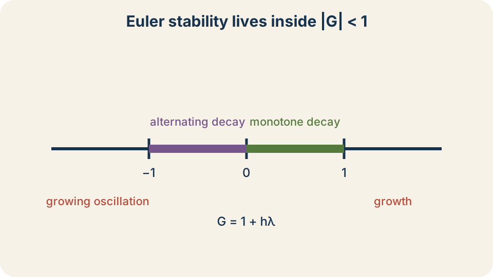
The amplification factor is $G=1+h\lambda$. Numerical decay requires $|G|<1$. Positive $G$ below one gives monotone decay, while negative $G$ above negative one gives alternating decay. At $G=-1$, magnitude no longer decreases. Outside the interval, Euler invents growth. Stability therefore constrains step size even before fine accuracy is considered.

Interpret Euler steps in a slope field

A slope field draws a short segment with slope $f(t,y)$ at many points. Euler’s method converts those visual directions into a path. Start at the initial condition, follow the local segment for horizontal distance $h$, and arrive at the next approximate point. Repeat using the slope field at the new location. The computed polygon should roughly follow the field’s directional texture.

The comparison can reveal errors. If the table says $y$ increases while the field at that point slopes downward, the slope evaluation or sign is wrong. If a step crosses an equilibrium solution unexpectedly, the step may be too large. If trajectories in the field bend sharply, smaller steps are appropriate. Visual and numerical representations should support each other.

Euler paths do not generally pass through the centers of all drawn segments because the grid and step points may differ. The field is a qualitative sampling of the same function $f$. The algorithm evaluates exact slope formulas at its own approximate points. Both representations encode the differential equation rather than the unknown solution formula. Their agreement is a conceptual check rather than an identity of drawings.

Preserve units in applied models

Suppose temperature $T$ is measured in degrees Celsius and time in minutes. In Newton’s cooling model $T'=-k(T-T_a)$, the constant $k$ has units $\mathrm{min}^{-1}$. The difference $T-T_a$ has degrees Celsius. The right side therefore has $\frac{^\circ\mathrm{C}}{\mathrm{min}}$, matching $T'$. Multiplying by step $h$ in minutes produces a temperature change.

Let $T_a=20.0\,{}^\circ\mathrm{C}$, $T_0=80.0\,{}^\circ\mathrm{C}$, $k=0.100\,\mathrm{min}^{-1}$, and $h=2.00\,\mathrm{min}$. The initial slope is $-0.100\,\mathrm{min}^{-1}(60.0\,{}^\circ\mathrm{C})=-6.00\,\frac{^\circ\mathrm{C}}{\mathrm{min}}$. The first increment is $(2.00\,\mathrm{min})(-6.00\,\frac{^\circ\mathrm{C}}{\mathrm{min}})=-12.0\,{}^\circ\mathrm{C}$. Therefore $T_1=68.0\,{}^\circ\mathrm{C}$. Units cancel correctly in the update.

An update that adds a rate directly to a state is dimensionally invalid. The step size supplies the missing independent-variable unit. If $h$ is given in seconds while $k$ is per minute, convert one before multiplying. Unit consistency can catch hidden scale factors of $60$. Numerical methods do not suspend physical dimensional reasoning.

Compare Euler with improved methods

Euler uses the slope at the beginning of each step. The midpoint method estimates a slope near the step’s center. Heun’s method averages beginning and predicted-ending slopes. Classical fourth-order Runge–Kutta combines four slope samples. These methods use additional work per step to achieve higher accuracy order.

A higher-order method is not automatically best in every setting. Cost per step, stability, available error control, discontinuities, and model complexity matter. Euler remains valuable for conceptual development, quick estimates, and certain simple simulations. Its limitations are visible and therefore pedagogically useful. It provides the baseline against which improved methods can be understood.

Adaptive methods change $h$ during computation. They shorten steps where the solution varies rapidly or error estimates grow. They lengthen steps where behavior is smooth. This allocates work according to local difficulty. The fixed-step Euler method introduces the principle before adaptive algorithms automate it.

Follow an error-resistant workflow

First write the differential equation as an explicit slope rule $y'=f(t,y)$ and record the initial condition. Choose a step whose units match the independent variable. Determine the number of steps needed to reach the target input. Build a table with current input, current state, slope, increment, and next state. Do not round aggressively inside the recurrence.

At each row, evaluate the slope at the current approximate point. Multiply by $h$ to obtain a state change. Add that change to obtain $y_{n+1}$, then advance time by $h$. Check the sign against the slope field or physical model. Repeat until the target is reached exactly or handle a shorter final step explicitly.

Then repeat with a smaller step size. Compare the target values and qualitative trajectory. Check stability conditions when rapid decay or stiffness is possible. Report step size and method with the answer because they define the approximation. A bare decimal without numerical-method context is incomplete evidence.

Repair common misconceptions

Euler’s method does not use the exact future slope. It uses the slope available at the current approximate state. Substituting $f(t_{n+1},y_{n+1})$ would define a different, implicit method. Reusing $f(t_0,y_0)$ for every step follows one tangent forever. Recalculation at each step is essential.

More decimal places do not imply greater accuracy. They may only display arithmetic performed on a coarse approximation. Step refinement or comparison with a higher-order solution provides actual evidence. Another mistake is to equate local $h^2$ error with final $h^2$ error. Euler’s accumulated global order is typically $h$ over a fixed interval.

Smaller steps usually improve truncation accuracy, but stability and finite precision still matter. A step within the stability interval can remain too coarse for accurate values. A step outside it can create fictitious oscillation or growth. Negative intermediate values are not always errors, but they may violate a model’s physical domain. Numerical output must be interpreted, not merely generated.

Retrieve and connect forward

For $y'=-4y$ with $h=0.500$, the amplification factor is $1-4(0.500)=-1$. Euler predicts alternating values of constant magnitude. The exact solution $y_0e^{-4t}$ decays toward zero. The step lies on the numerical stability boundary. This example separates an algebraically valid recurrence from a physically misleading approximation.

For $y'=y$, smaller positive steps move the Euler estimate of $y(1)$ toward $e$. The method underestimates because the exact exponential is concave up and tangent steps lie below it. Local truncation error scales like $h^2$, while typical global error scales like $h$. A refinement table turns these statements into observable evidence. The calculation should be accompanied by its step size.

Euler’s method converts a slope rule into a trajectory one step at a time. It makes the definition of a differential equation computationally concrete. Error analysis shows why local approximation does not guarantee global accuracy. Stability analysis shows why a decaying differential equation can produce a growing numerical sequence. Higher-order and adaptive methods retain this stepwise logic while using slope information more effectively.