Equilibria Organize Autonomous ODEs

Many differential equations are difficult or impossible to solve in a simple closed form. Their long-term behavior can still be understandable. Equilibrium solutions divide the state line into regions where solutions rise or fall. A phase line compresses this information into arrows. Stability then asks how nearby solutions respond to disturbance.

An equilibrium does not mean every microscopic process has stopped. It means the modeled state variable has zero net rate of change. Population births may balance deaths, heat input may balance heat loss, or chemical production may balance removal. Different mechanisms can remain active. The differential equation records their net effect.

This article develops autonomous first-order equations of form $y'=f(y)$. It explains how to find equilibria, build sign charts, classify stability, use linearization, handle inconclusive cases, and follow parameter changes. Examples emphasize prediction without explicit solution formulas. Diagrams connect slope fields, phase lines, and solution curves. The central idea is that zeros and signs organize dynamics.

Autonomous equations and state-dependent rates

An autonomous equation has form $\frac{dy}{dt}=f(y)$. The independent variable $t$ does not appear explicitly on the right. Rate depends only on current state $y$. Two solutions passing through the same state encounter the same derivative under the model. Time translation does not change the rule.

The prime notation $y'$ abbreviates $\frac{dy}{dt}$. It represents instantaneous rate of change of state with respect to time. If $y'>0$, the solution rises as $t$ increases. If $y'<0$, it falls. If $y'=0$, its graph has horizontal tangent at that state.

Units must balance. If $y$ is measured in people and $t$ in years, then $f(y)$ has unit $\mathrm{\frac{people}{year}}$. Parameters inside $f$ carry units that make every term consistent. A sign diagram suppresses units visually but does not remove them. Interpretation should restore them.

Equilibrium means a constant solution

An equilibrium value $y^*$ satisfies $f(y^*)=0$. The star labels a special state rather than an exponent. If $y(t)=y^*$ for all $t$, then its derivative is zero. Substitution gives $0=f(y^*)$. Thus the constant function is a solution.

Finding a root of $f$ is necessary and sufficient for an equilibrium in this scalar autonomous setting. Do not solve $f'(y)=0$ instead. Roots of $f'$ locate extrema of the rate function. They need not be constant solutions. The original differential equation supplies the equilibrium condition.

For $y'=y(1-y)$, roots are $y=0$ and $y=1$. Therefore $y(t)=0$ and $y(t)=1$ are equilibrium solutions. A nonconstant solution may approach either level. It cannot be called an equilibrium merely because its derivative becomes small. Exact zero rate at the constant state is required.

Equilibrium is not ordinary algebraic equality

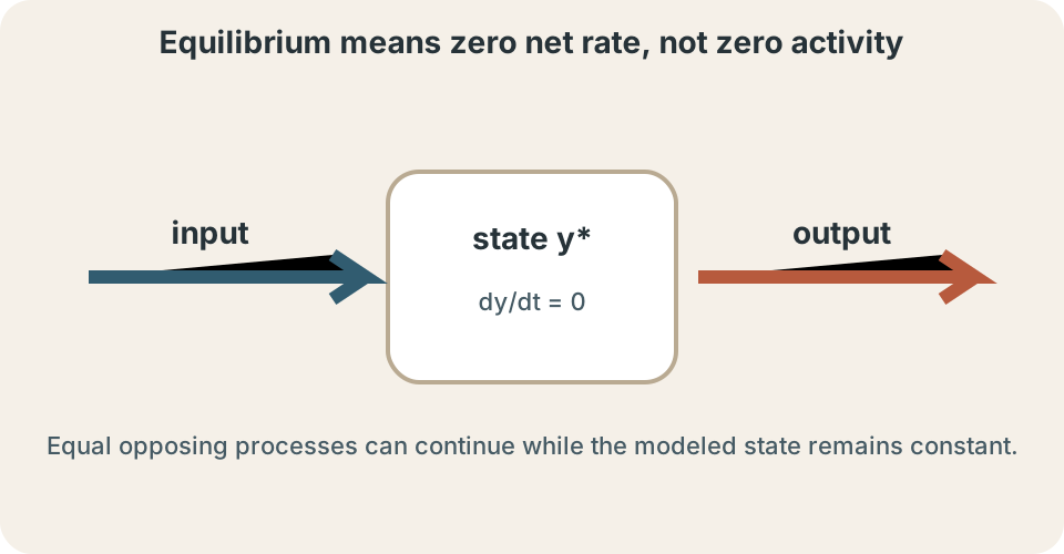
The equation $f(y^*)=0$ identifies a state where net rate vanishes. It does not say the state variable itself must be zero. A thermal equilibrium can occur at $y^*=22\,^\circ\mathrm C$. A population equilibrium can occur at $y^*=5000$ organisms. Zero rate and zero state are different quantities.

The state can remain constant even while components exchange. In a tank, inflow may equal outflow. In a population, births may equal deaths. In a chemical reactor, formation may equal removal. The model collapses those competing processes into $f(y^*)=0$.

An equilibrium is defined relative to the model boundary and variables. Adding an omitted process can shift or remove it. A constant state in one variable may coexist with change in an unmodeled variable. Scientific interpretation should name what is held steady. Mathematical classification follows the stated equation.

Build a phase line from roots and signs

Begin by solving $f(y)=0$. Mark every real root on a line representing the state axis. Those points divide the line into intervals. If $f$ is continuous and has no root inside an interval, its sign cannot change there. One test value determines the arrow for that entire interval.

Where $f(y)>0$, draw an arrow toward increasing $y$. On a vertical phase line, that arrow points upward. Where $f(y)<0$, draw an arrow toward decreasing $y$. The phase line does not display time directly. It displays state direction as time moves forward.

The sign chart is an algebraic foundation for the arrows. Factorization can reveal signs efficiently. Repeated roots require special care because sign may or may not change across them. Test intervals rather than assuming alternation. The arrows are conclusions, not decoration.

Stability describes response to disturbance

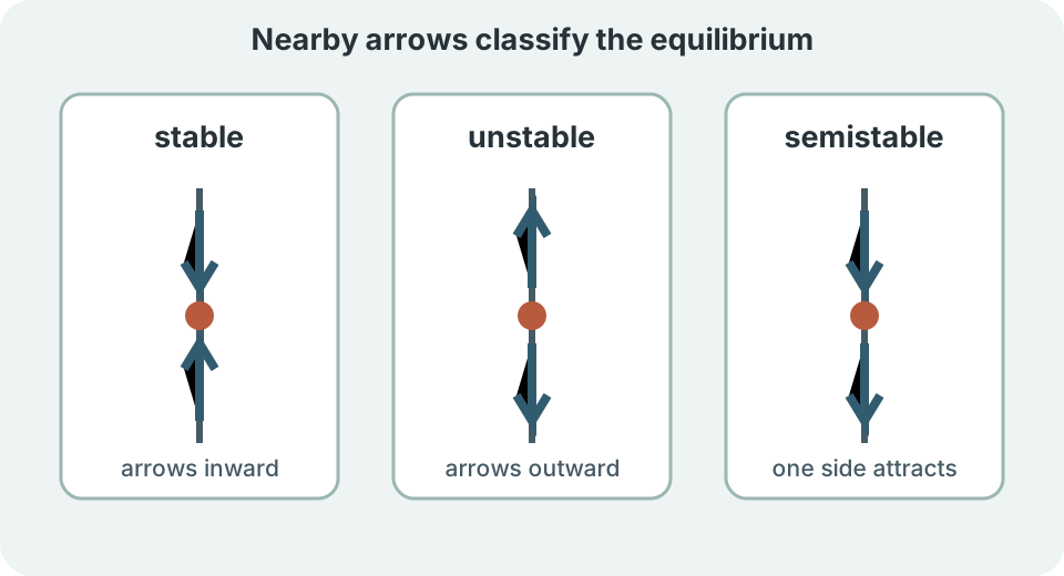
An equilibrium is locally asymptotically stable when sufficiently nearby solutions remain nearby and approach it as time increases. On a one-dimensional phase line, arrows point toward it from both sides. The word “local” restricts the claim to a neighborhood. Farther initial conditions may behave differently. Nearby response defines the classification.

An equilibrium is unstable when arbitrarily small disturbances can move away. On the phase line, arrows point away on at least one side for the common scalar classifications. A repeller has arrows away on both sides. Instability does not mean every initial condition immediately diverges. The exact equilibrium solution itself remains constant.

A semistable equilibrium attracts from one side and repels from the other. One arrow points toward it while the other also points in the same state direction, crossing conceptually around the root only if uniqueness allows. The equilibrium is not asymptotically stable in a two-sided neighborhood. One-sided behavior must be stated explicitly. A single label should not hide that asymmetry.

A complete cubic phase-line example

Consider $\frac{dy}{dt}=y(1-y)(y-2)$. The factored form reveals equilibria $y^*=0,1,2$. These values partition the state line into four intervals. Choose one test value in each interval. Determine only the sign of each factor.

For $y<0$, the three factor signs are negative, positive, and negative, giving positive product. For $0<y<1$, signs are positive, positive, and negative, giving negative product. For $1<y<2$, signs are positive, negative, and negative, giving positive product. For $y>2$, signs are positive, negative, and positive, giving negative product. The four tests cover every nonequilibrium state.

Arrows therefore point upward, downward, upward, and downward across successive intervals. They point toward $0$ from both sides, so zero is stable. They point away from $1$, so one is unstable. They point toward $2$, so two is stable. Classification follows from adjacent arrows rather than root size.

Predict trajectories without solving

Suppose $y(0)=1.4$. This state lies in interval $(1,2)$ where $f(y)>0$. The solution increases. The equilibrium at $2$ forms an upper boundary under standard uniqueness conditions. The trajectory approaches $2$ rather than crossing it.

Suppose $y(0)=0.4$. This lies in $(0,1)$ where derivative is negative. The solution decreases toward zero. It cannot cross equilibrium zero under uniqueness. Its long-term limit is predicted from arrows and barriers.

Suppose $y(0)>2$. Derivative is negative and the state falls toward two. Initial values below zero have positive derivative and rise toward zero. The unstable value one separates two basins of attraction. A basin is the set of initial states approaching one attractor.

Why equilibria act as barriers

If $f$ satisfies conditions ensuring local uniqueness, two solution curves cannot intersect in the time–state plane. An equilibrium is itself a solution curve. A nonconstant solution reaching it at finite time would intersect that constant solution. Uniqueness would then force both to be the same solution through that point. This contradiction prevents ordinary crossing.

This reasoning often prevents crossing. A trajectory can approach an equilibrium asymptotically as $t\to\infty$. It may take arbitrarily long to arrive. The phase line therefore treats equilibrium points as boundaries between solution families. Sign arrows alone gain strength from uniqueness.

If uniqueness fails, unusual behavior can occur. Solutions may reach an equilibrium and wait before departing in equations with insufficient regularity. Therefore barrier language needs hypotheses. A common sufficient condition is local Lipschitz continuity of $f$. Introductory smooth polynomial examples satisfy it.

The derivative stability test

Suppose $f$ is differentiable and $f(y^*)=0$. If $f'(y^*)<0$, the graph of $f$ crosses the axis with negative slope. Just left of the root, $f$ is typically positive. Just right, it is negative. Arrows point inward.

Therefore $f'(y^*)<0$ implies local asymptotic stability in the standard scalar setting. If $f'(y^*)>0$, signs reverse. Left side has negative rate and right side positive rate. Arrows point outward, giving instability. The derivative’s sign encodes the local crossing direction.

The derivative test is local. It says nothing by itself about distant initial conditions. It also requires a hyperbolic equilibrium, meaning $f'(y^*)\ne0$. When the derivative equals zero, the test is inconclusive. Return to the exact sign diagram.

Why linearization explains the test

Near equilibrium, write $y=y^*+u$, where $u$ is a small perturbation. Taylor expansion gives $f(y^*+u)\approx f(y^*)+f'(y^*)u$. Because $f(y^*)=0$, the approximation becomes $u'\approx f'(y^*)u$. This is a linear equation. Variable $u$ measures signed distance from equilibrium.

Its solution is $u(t)\approx u(0)e^{f'(y^*)t}$. If $f'(y^*)<0$, the exponential decays toward zero. The perturbation shrinks. If $f'(y^*)>0$, the exponential grows. The perturbation expands.

The approximation neglects higher-order terms. When the linear coefficient is nonzero, it dominates sufficiently near equilibrium. When it is zero, higher powers determine behavior. That is why zero derivative cannot decide stability. The nonlinear sign must be examined.

Inconclusive derivative test and semistability

Consider $y'=y^2$. Equilibrium is $y^*=0$. Derivative of rate function is $f'(y)=2y$, so $f'(0)=0$. Linearization gives only $u'\approx0$. It misses the leading quadratic behavior.

For every nonzero $y$, $y^2>0$. Arrows point toward increasing state on both sides. Negative initial states rise toward zero. Positive initial states rise away and can blow up in finite time. Zero is semistable.

Now consider $y'=-y^3$. Rate is positive for negative $y$ and negative for positive $y$. Arrows point toward zero from both sides. Although $f'(0)=0$, equilibrium is asymptotically stable. These two examples prove that the zero derivative case needs sign analysis.

Repeated roots predict sign behavior

For a factored polynomial rate, root multiplicity helps anticipate sign changes. A factor $(y-a)^m$ changes sign across $a$ when $m$ is odd. It keeps the same sign when $m$ is even. Other nonzero factors contribute a fixed local sign. This pattern resembles polynomial graph crossings and touches.

An odd simple root often yields stable or unstable behavior because arrows reverse direction across it. An even root often yields semistability because arrows retain the same direction. The surrounding factor sign determines which side attracts. Multiplicity is a clue, not a substitute for checking all factors. A test point confirms the anticipated pattern.

For $y'=(y-1)^2(y+2)$, equilibrium $1$ has even multiplicity. Near one, factor $y+2$ is positive, so rate is positive on both sides. The state increases toward one from below and away above. Equilibrium one is semistable. Its attraction occurs only from the lower side.

Slope fields and phase lines are related

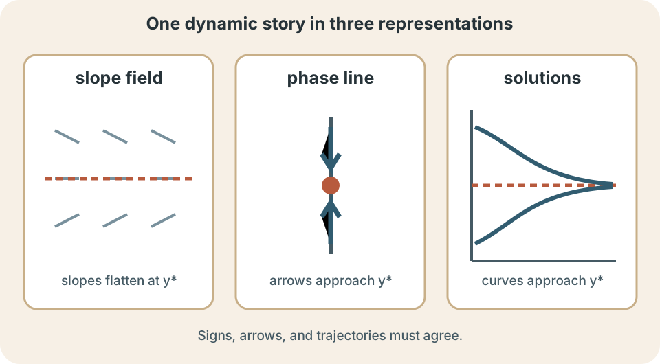
In an autonomous slope field, slope depends only on vertical coordinate $y$. Along each horizontal row, small line segments have the same slope. Equilibrium levels appear as horizontal rows of zero slope. Positive rows tilt upward. Negative rows tilt downward.

The phase line extracts only the vertical direction information. It discards time position and slope magnitude. This compression makes long-term structure easier to see. The slope field retains more local shape information. The two representations should agree.

Solution curves cannot cross each other under uniqueness. They bend according to changing row slopes. Near a stable equilibrium, curves flatten as they approach. Near an unstable equilibrium, nearby curves peel away. Sketching both representations reinforces the model.

Logistic growth as a physical model

The logistic equation is $\frac{dP}{dt}=rP\left(1-\frac{P}{K}\right)$. Population $P$ may be measured in organisms, time in years, $r$ in $\mathrm{\frac{1}{year}}$, and carrying capacity $K$ in organisms. The fraction $\frac{P}{K}$ is dimensionless. Equilibria satisfy $P=0$ or $P=K$. Both values make the modeled net growth rate zero.

For $r>0$ and $0<P<K$, both factors are positive, so population grows. For $P>K$, the second factor is negative, so population decreases. For physically meaningful $P>0$, arrows point toward $K$. Carrying capacity is stable. The conclusion assumes constant positive parameters.

Equilibrium zero is unstable for positive populations because small positive states grow away. Mathematically negative states may appear, but they are not meaningful population sizes. The physical domain restricts interpretation. Stability can be one-sided at a domain boundary. Model meaning therefore filters mathematical states.

Harvesting introduces thresholds

Add constant harvest $H$ to obtain $\frac{dP}{dt}=rP\left(1-\frac{P}{K}\right)-H$. Equilibria are intersections of the concave-down growth curve with horizontal level $H$. Depending on $H$, there can be two, one, or no nonnegative equilibria. A parameter changes the phase portrait. Harvest has unit $\mathrm{\frac{organisms}{year}}$ in this model.

When harvest is below the maximum natural growth rate, two equilibria exist. The lower is typically unstable and acts as a threshold. The upper is stable. A population pushed below the threshold declines rather than recovering. This is an Allee-like management threshold created by harvesting.

At the critical harvest, the two equilibria merge into a repeated root. Above it, no equilibrium remains and the model predicts decline across the physical region. This qualitative change is a saddle-node bifurcation. Parameter awareness turns a static phase line into a family of behaviors. The threshold has direct management significance.

Newton cooling as a balance model

Newton’s cooling model is $\frac{dT}{dt}=-k(T-T_a)$ with $k>0$. Temperature $T_a$ is ambient temperature. Equilibrium satisfies $T=T_a$. If the object is hotter, $T-T_a>0$ and derivative is negative. It cools.

If the object is colder, $T-T_a<0$ and derivative is positive. It warms. Arrows point toward ambient temperature from both sides. The derivative test gives $f'(T_a)=-k<0$. The equilibrium is stable.

The model assumes ambient temperature remains constant and heat-transfer rate is proportional to the difference. A changing environment makes the equation nonautonomous. Radiation and phase changes may violate linear proportionality. Stability conclusions belong to the stated model and conditions. Approximation quality depends on the temperature range.

Equilibria versus turning points

An equilibrium solution is constant for all modeled time. A turning point of one nonconstant solution is a moment where its derivative is zero. In a scalar autonomous equation with uniqueness, a nonconstant solution generally cannot have an ordinary turning point at an equilibrium state and then continue through. The zero-rate state is a barrier. Constant and momentary behavior must not be conflated.

In a nonautonomous equation $y'=f(t,y)$, zero derivative may occur at isolated times without creating a constant solution. The right side can change because time changes. Solving $f(t,y)=0$ produces a null-slope curve rather than necessarily an equilibrium. Autonomous and nonautonomous language should not be mixed. A constant solution must satisfy the equation for every time.

In second-order motion, velocity can be zero at a turning point while acceleration is nonzero. The full state includes position and velocity. Equilibrium requires all state derivatives to vanish. One component being momentarily zero is insufficient. State definition controls the concept.

Stability has several meanings

Lyapunov stability means nearby initial states remain nearby for future time. Asymptotic stability adds convergence to the equilibrium. Exponential stability requires a specific exponential decay bound. These concepts are related but not identical. Introductory phase-line “stable” often means asymptotically stable.

An equilibrium with $y'=0$ for every $y$ is Lyapunov stable but not asymptotically stable. Every initial state remains where it began. None approaches a different equilibrium. Arrows are absent everywhere. This neutral case prevents an overly broad inward-arrow slogan.

Global asymptotic stability means every allowed initial state approaches the equilibrium. A local sign test cannot prove global behavior unless the entire domain is analyzed. Other equilibria or finite-time escape can prevent it. State the domain and scope of each stability claim. Global is a stronger word than local.

Parameter-dependent equilibria

Consider $y'=\mu-y^2$, where $\mu$ is a parameter. For $\mu>0$, equilibria are $y^*=\pm\sqrt{\mu}$. Derivative $f'(y)=-2y$ makes positive root stable and negative root unstable. For $\mu=0$, they merge at zero. The repeated equilibrium is nonhyperbolic.

For $\mu<0$, no real equilibrium exists because $\mu-y^2<0$ for every real $y$. All arrows point downward. Crossing $\mu=0$ changes the number and type of equilibria. This is another saddle-node pattern. A bifurcation diagram plots equilibrium values against parameter.

Parameter units must make $\mu$ compatible with $y^2$ inside the rate expression. Rescaling can produce dimensionless normal forms. The normal form captures qualitative behavior shared by many models. Application-specific variables then restore units and interpretation. Structural similarity is a key benefit of dynamical-systems analysis.

Numerical simulations need equilibrium checks

A numerical method approximates trajectories at discrete times. Step size can affect apparent stability. A large explicit Euler step can oscillate or diverge around a truly stable equilibrium. Numerical artifacts should not be mistaken for model dynamics. Compare with the phase-line prediction.

For linearized equation $u'=au$ with $a<0$, Euler update is $u_{n+1}=(1+a\Delta t)u_n$. Numerical decay requires suitable size of $\Delta t$. If the multiplier has magnitude greater than one, the discrete approximation grows. The continuous solution still decays. This mismatch is numerical instability.

Equilibria should remain fixed under a consistent numerical method because $f(y^*)=0$. Roundoff and solver tolerance can cause tiny departures. Residual $|f(y^*)|$ checks a computed root. Convergence studies distinguish time-step error from modeled behavior. Qualitative analysis guides numerical trust.

Common misconceptions and repairs

One misconception solves $f'(y)=0$ to find equilibria. The correct equation is $f(y)=0$. Derivative $f'$ is used later for a stability test. Keep the rate function and its slope distinct. Substitute candidate equilibrium into the original ODE.

Another misconception labels every zero derivative as stable. Stability depends on nearby arrows. A root can attract, repel, or do one of each. Build a sign chart. The value zero alone supplies no classification.

A third misconception assumes the derivative test always decides. When $f'(y^*)=0$, linear terms vanish. Higher-order behavior matters. Test signs on both sides. State semistability or nonlinear stability precisely.

A reliable phase-line routine

Write the equation in autonomous form $y'=f(y)$. State the meaningful state domain and parameter assumptions. Solve $f(y)=0$ exactly when possible. Mark all real allowed equilibria. Factor the rate function if useful.

Choose one test point in every interval. Record the sign of $f$. Draw arrows toward greater state for positive sign and toward lesser state for negative sign. Classify each equilibrium from both adjacent arrows. Use $f'(y^*)$ as a check when nonzero.

Select an initial condition and locate its interval. Predict monotonic direction, barriers, and possible long-term limit. Check units and physical domain. Note whether the conclusion is local or global. Use explicit solutions or numerics afterward for quantitative timing.

Further deductions and connection forward

For $y'=y^2$, zero is semistable because arrows point upward on both sides. For $y'=-y$, zero is globally asymptotically stable on the real line. For $y'=y$, zero is unstable. These three simple rates generate three distinct patterns. Their signs carry the essential information.

Without solving, analyze $y'=y(y-3)^2$. Equilibria are zero and three. Sign changes across zero but not across three. Testing intervals shows which state attracts from each side. The repeated root warns that the linear test at three will be inconclusive.

Equilibrium analysis extends into two-dimensional phase planes. There, nullclines locate where individual derivatives vanish, and Jacobian eigenvalues classify many equilibria locally. Bifurcation theory studies how classifications change with parameters. The one-dimensional phase line is the conceptual foundation. Its habits of roots, signs, and nearby response continue forward.