Phase Planes Show the Geometry of Two-State Systems

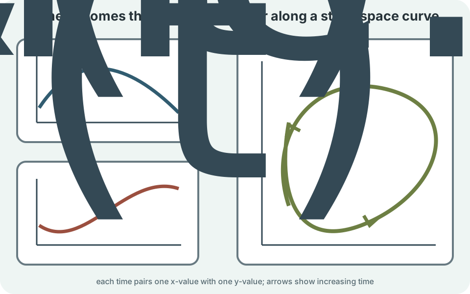
A phase plane represents the complete state of a two-variable autonomous system. For $x'=f(x,y)$ and $y'=g(x,y)$, the ordered pair $(x,y)$ is one state. The vector $(f(x,y),g(x,y))$ gives the state’s instantaneous direction of change. A solution becomes a curve traced through the $xy$-plane. Time controls motion along the curve even though it is not drawn as an axis.

This representation differs from ordinary graphs of $x(t)$ and $y(t)$. A time plot shows each variable against time on separate vertical scales. A phase portrait plots one state variable against the other. It emphasizes geometry, long-term behavior, and dependence on initial condition. Several trajectories can be displayed at once without adding a third time dimension.

This article builds a method for reading and constructing phase portraits. It explains vector fields, nullclines, equilibria, trajectory direction, nonintersection, linear systems, eigenvalue classification, and linearization. Worked examples connect algebraic calculations to geometric features. Invariant regions and physical constraints keep interpretation tied to models. The goal is to reason about dynamics even when explicit formulas are unavailable.

State space records all needed variables

A dynamical state contains enough information to predict future evolution under the model. In a population system, $x$ and $y$ might be two species populations. In an oscillator, $x$ can be position and $y$ can be velocity. In a compartment model, they can be two amounts or concentrations. The meaning and units of axes come from the application.

For the autonomous system $x'=f(x,y)$ and $y'=g(x,y)$, the right sides do not contain time explicitly. The prime means differentiation with respect to time. The function $f$ has units of $x$ per time, and $g$ has units of $y$ per time. Their vector is tangent to the solution trajectory. Autonomous systems assign the same direction whenever the same state is revisited.

An initial condition $(x(0),y(0))=(x_0,y_0)$ selects one trajectory. The symbols $x_0$ and $y_0$ identify the starting state. Nearby initial conditions can approach similar or dramatically different long-term behavior. A phase portrait samples this family. It is not one single solution.

The vector field gives local motion

At a point $(x,y)$, draw a small arrow proportional or parallel to $(f(x,y),g(x,y))$. Its horizontal component is $x'$. Its vertical component is $y'$. Rightward arrows mean $x$ increases, and leftward arrows mean $x$ decreases. Upward arrows mean $y$ increases, and downward arrows mean $y$ decreases.

Arrow length can represent speed through state space, $\sqrt{(x')^2+(y')^2}$, but many plots normalize lengths so direction remains readable. A normalized field hides relative speed. The arrow orientation still identifies tangent direction. Plot settings must therefore be stated. Visual appearance can encode or suppress information.

The trajectory slope where $x'\ne0$ is $\frac{dy}{dx}=\frac{y'}{x'}=\frac{g(x,y)}{f(x,y)}$. This eliminates time locally. A vertical tangent occurs where $x'=0$ and $y'\ne0$. A horizontal tangent occurs where $y'=0$ and $x'\ne0$. Equilibria require both components zero.

Nullclines partition the plane

The $x$-nullcline is the set where $x'=f(x,y)=0$. Along it, the vector field has no horizontal component. Arrows are vertical unless $y'$ also vanishes. The $y$-nullcline is the set where $y'=g(x,y)=0$. Along it, arrows are horizontal unless the state is an equilibrium.

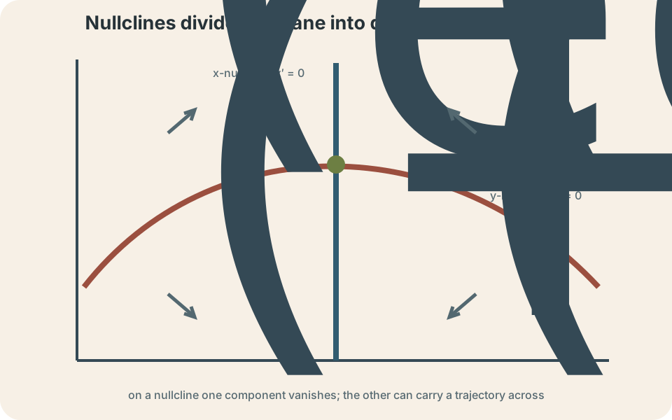
Nullclines divide the plane into regions where component signs are constant or at least easier to determine. Test one point in each region. Record the sign pair $(\operatorname{sgn}x',\operatorname{sgn}y')$. The four possibilities correspond to northeast, southeast, northwest, and southwest motion. This sign chart provides a qualitative portrait before any numerical integration.

An equilibrium occurs at an intersection of nullclines. There $x'=0$ and $y'=0$, so the state remains fixed. Not every nullcline point is an equilibrium. On one nullcline, only one component stops instantaneously. The system can cross that curve in the other direction.

Trajectories follow arrows but do not equal them

A vector field contains local velocity information at every point. A trajectory is an integral curve whose tangent matches that field at every point it visits. One arrow does not show an entire future. Following successive directions constructs the path. Numerical solvers approximate this process in time steps.

Arrows indicate orientation along a trajectory. A curve without arrows can conceal whether the state approaches or leaves an equilibrium. Add several arrows when direction might be ambiguous. Time generally passes unevenly along the drawn curve if arrow lengths are normalized. Geometry and timing are related but not identical.

Trajectories of a well-posed autonomous system cannot ordinarily cross at a non-equilibrium point. A crossing would assign two future tangent directions to the same state, contradicting uniqueness. Curves can approach one another and can share an equilibrium asymptotically. Apparent crossings in a rough plot may be graphical artifacts. Uniqueness turns geometry into a diagnostic.

Equilibrium stability is a neighborhood property

An equilibrium is stable in the Lyapunov sense if trajectories starting sufficiently near remain near. It is asymptotically stable if they also approach the equilibrium as time increases. It is unstable if arbitrarily close initial states can move away beyond a chosen neighborhood. These definitions concern all nearby directions. One approaching trajectory does not prove stability.

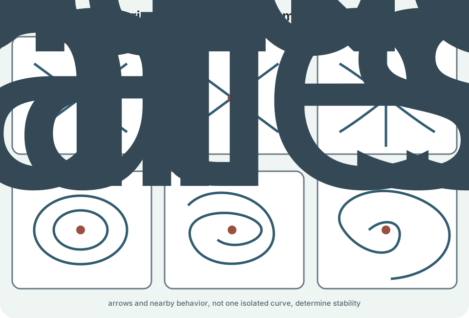
A sink attracts nearby trajectories forward in time. A source repels them. A saddle attracts along some directions and repels along others, making it unstable overall. A center is surrounded by closed trajectories in an ideal linear conservative system. A spiral combines rotation with inward or outward radial behavior.

Stability can be local or global. Local analysis describes a neighborhood. A locally attracting equilibrium may coexist with another attractor elsewhere. Separatrices can divide basins of attraction. Initial condition determines which long-term behavior occurs.

Linear systems organize the basic patterns

A linear autonomous system is $\mathbf u'=A\mathbf u$, where $\mathbf u=\begin{bmatrix}x\\y\end{bmatrix}$ and $A$ is a constant $2\times2$ matrix. Matrix multiplication gives the two component equations. The origin is always an equilibrium. Other equilibria can occur if $A$ is singular. Eigenvalues and eigenvectors organize its trajectories.

If $A\mathbf v=\lambda\mathbf v$, then a solution along eigenvector $\mathbf v$ is $\mathbf u(t)=Ce^{\lambda t}\mathbf v$. The scalar $\lambda$ is the eigenvalue, $\mathbf v$ is an eigenvector, and $C$ selects initial magnitude. Positive real $\lambda$ produces growth forward in time. Negative real $\lambda$ produces decay. The eigenvector line remains invariant because the derivative stays parallel to that direction.

With two independent real eigenvectors, general solution is a linear combination of two modal solutions. Their relative rates determine trajectory shape. An initial condition exactly on one eigenvector remains on that line. Those invariant lines anchor the portrait. Most initial conditions combine both modes.

Classify real-eigenvalue equilibria

Two negative real eigenvalues produce a stable node or sink. Both modal components decay. Trajectories approach the origin, often tangent eventually to the slower-decaying eigenvector. The eigenvalue closer to zero decays more slowly. Its direction dominates at late time.

Two positive real eigenvalues produce an unstable node or source. Both modes grow forward in time. Trajectories leave the origin. Backward in time, the same state approaches it. Stability always specifies time direction.

Real eigenvalues with opposite signs produce a saddle. The negative-eigenvalue direction is stable, and the positive-eigenvalue direction is unstable. The invariant eigenvector lines form special trajectories. Nearby off-axis trajectories eventually leave along the unstable direction. A saddle is unstable despite having an attracting path.

Complex eigenvalues produce rotation with growth or decay

Complex-conjugate eigenvalues have form $\lambda=a\pm ib$. The real part $a$ controls exponential growth or decay. The imaginary part $b$ controls angular oscillation in state space. If $a<0$, trajectories spiral inward. If $a>0$, they spiral outward.

If $a=0$ and $b\ne0$ in an ideal linear system, trajectories are typically closed curves around a center. Their amplitude remains constant. A small dissipative change can turn a center into a spiral sink. Centers are therefore structurally delicate. Nonlinear systems require additional analysis.

The sign of rotation is not determined by eigenvalues alone. Evaluate the vector field at a convenient point, such as $(1,0)$. If the arrow points upward there, rotation begins counterclockwise. If it points downward, rotation begins clockwise. One local direction determines orientation around the equilibrium.

Trace and determinant offer a quick classification

For matrix $A=\begin{bmatrix}a&b\\c&d\end{bmatrix}$, trace is $\operatorname{tr}A=a+d$. Determinant is $\det A=ad-bc$. Eigenvalues satisfy $\lambda^2-(\operatorname{tr}A)\lambda+\det A=0$. The discriminant is $(\operatorname{tr}A)^2-4\det A$. These quantities classify many linear systems.

If $\det A<0$, eigenvalues have opposite signs and the origin is a saddle. If $\det A>0$ and the discriminant is positive, eigenvalues are real with the same sign determined by trace. Negative trace gives a sink, and positive trace gives a source. If the discriminant is negative, eigenvalues are complex. Trace sign again determines inward or outward spiraling.

The trace–determinant plane is a summary tool, not a replacement for eigenvectors or nonlinear reasoning. It does not show invariant directions. Repeated eigenvalues can create distinct cases depending on eigenvector completeness. Zero determinant or trace can sit on boundaries requiring separate treatment. Classification must note degeneracies.

Worked linear example

Consider $x'=x+2y$ and $y'=2x+y$. The matrix is $A=\begin{bmatrix}1&2\\2&1\end{bmatrix}$. Its characteristic equation is $\det(A-\lambda I)=0$. Expansion gives $(1-\lambda)^2-4=0$. The eigenvalues are $\lambda_1=3$ and $\lambda_2=-1$.

Opposite signs identify a saddle. For $\lambda_1=3$, an eigenvector is $\begin{bmatrix}1\\1\end{bmatrix}$. For $\lambda_2=-1$, an eigenvector is $\begin{bmatrix}1\\-1\end{bmatrix}$. The line $y=x$ is unstable forward in time. The line $y=-x$ is stable.

At $(1,0)$, vector is $(1,2)$, pointing right and upward. At $(0,1)$, vector is $(2,1)$. These samples agree with departure toward the unstable line for generic forward trajectories. An initial condition exactly on $y=-x$ approaches the origin. Any small component along $y=x$ eventually grows.

Nullcline example for a nonlinear system

Consider $x'=x(1-x-y)$ and $y'=y(2-x-y)$. The $x$-nullclines are $x=0$ and $1-x-y=0$. The $y$-nullclines are $y=0$ and $2-x-y=0$. Their intersections in relevant regions give equilibria. Population interpretation restricts attention to $x\ge0$ and $y\ge0$.

On an axis, the corresponding factor keeps that variable derivative zero. Thus the coordinate axes are invariant. A trajectory beginning with a nonnegative population cannot cross through an axis under uniqueness. Sign tests between nullclines show where each population increases or decreases. The portrait can be sketched without explicit solutions.

The two slanted nullclines are parallel and do not intersect. Equilibria occur on axes at selected intercepts and at the origin. Linearization can classify them locally. Boundary equilibria matter because the model allows extinction of one population. Physical domain constraints are part of the phase plane.

Linearization approximates nonlinear systems locally

For $\mathbf u'=\mathbf F(\mathbf u)$ with equilibrium $\mathbf u_*$, write a small displacement $\boldsymbol{\eta}=\mathbf u-\mathbf u_*$. The first-order approximation is $\boldsymbol{\eta}'=J(\mathbf u_*)\boldsymbol{\eta}$. The matrix $J$ is the Jacobian of partial derivatives. It describes the local linear response. Higher-order terms are neglected.

For $\mathbf F=(f,g)$, the Jacobian is $J=\begin{bmatrix}f_x&f_y\\g_x&g_y\end{bmatrix}$. Subscripts denote partial derivatives. Evaluate at the equilibrium before finding eigenvalues. If eigenvalues have nonzero real parts, their signs often determine local stability. This is the hyperbolic case.

If an eigenvalue has zero real part, linearization can be inconclusive. A nonlinear term may determine stability. A linear center can become an inward or outward nonlinear spiral. One must use other tools such as Lyapunov functions, higher-order analysis, or direct estimates. “Zero real part” is a signal to pause rather than declare neutral stability.

Nullclines are not usually trajectories

A nullcline is defined by one derivative component being zero. The other component can carry the state across it. For example, on an $x$-nullcline the arrow is vertical. Unless the curve itself is vertical or invariant for another reason, the trajectory crosses. Treating every nullcline as a solution curve is incorrect.

An invariant curve has vector field tangent to it everywhere. Coordinate axes in factored population models are common examples. An eigenvector line in a linear system is another. Invariance requires a directional condition, not merely one zero component. Check whether the field points along the curve.

Nullclines still guide trajectory shape. They mark vertical or horizontal tangencies. Crossing one can change the sign of a derivative. A local maximum of $x(t)$ can occur when a trajectory crosses the $x$-nullcline. Geometry connects directly to time-series turning points.

Invariant regions constrain behavior

An invariant region is a set that trajectories cannot leave forward in time. To verify one, examine the vector field on each boundary. It must point inward or tangent, not outward. Physical nonnegativity regions often have this property. Such reasoning can prove boundedness without solving the system.

Suppose a population model has $x'=xF(x,y)$. On $x=0$, derivative is zero, so the axis is invariant. Uniqueness prevents a positive solution from crossing into negative $x$. The same can hold for $y$. The first quadrant then remains physically meaningful.

Trapping regions can imply long-term behavior. If trajectories enter a bounded region and cannot leave, unbounded growth is excluded there. Additional theorems may establish an equilibrium or periodic orbit. Boundary arrows provide global information. Local eigenvalues alone cannot do that.

Oscillators reveal phase-plane meaning

A second-order equation $x''+\omega_0^2x=0$ becomes the system $x'=v$ and $v'=-\omega_0^2x$. Position $x$ and velocity $v$ form the state. Trajectories are closed ellipses. They represent periodic oscillation with constant mechanical energy. The origin is a center.

Adding damping gives $x'=v$ and $v'=-\omega_0^2x-2\gamma v$. For positive damping parameter $\gamma$, mechanical energy decreases. Trajectories spiral toward the origin when underdamped. Stronger damping can produce nonspiraling node behavior. Phase geometry displays qualitative regimes.

At a point with $x>0$ and $v=0$, acceleration is negative. The vector points downward in the $(x,v)$ plane. This establishes clockwise rotation under the conventional axis placement. The state is at a turning point in position but not at equilibrium. Equilibrium requires both position and velocity zero.

Phase portraits and numerical computation

Numerical solvers generate trajectories from selected initial conditions. A phase portrait should include enough starting points to reveal basins, separatrices, and attractors. Too few can hide behavior. Too many can obscure direction. The vector field and nullclines provide structure for choosing samples.

Step size and solver choice affect accuracy. A crude method can introduce artificial damping or growth in a conservative oscillator. Long-time closed orbits are especially sensitive. Compare numerical results with conserved quantities when available. Computation requires validation.

Plot windows can also mislead. A sink may appear global when another equilibrium lies outside the frame. A slowly changing vector field can look stationary. Axes with unequal scales distort angles and apparent spirals. Label units and scales.

Common mistakes and repairs

One mistake is treating the phase plane as a graph of $y$ as an ordinary function of $x$. Trajectories can have vertical tangents and closed loops. Both coordinates depend on time. Use parametric thinking. The curve records state evolution.

Another mistake is classifying stability from one visible trajectory. Examine a full neighborhood. A saddle attracts along one line but is unstable overall. Draw trajectories on both sides of invariant directions. Stability quantifiers concern all sufficiently close initial conditions.

A third mistake is calling nullclines solution curves automatically. Evaluate the other derivative. Check whether the vector field is tangent to the curve. Mark only true invariant sets as uncrossable. Use nullclines primarily for sign regions and tangencies.

A reliable phase-plane workflow

First define variables, units, physical domain, and time direction. Find equilibria by solving $f=0$ and $g=0$ simultaneously. Draw both nullclines. Create a sign chart in the regions they determine. Add representative field arrows.

Second analyze local stability. For a linear system, compute eigenvalues and eigenvectors. For a nonlinear system, form the Jacobian at each equilibrium. Identify cases where linearization is inconclusive. Mark invariant directions and expected rotation.

Third sketch trajectories without crossing and add arrows. Respect invariant boundaries and physical constraints. Use numerical trajectories to refine the portrait, not replace reasoning. Check the picture against time plots, conserved quantities, or limiting behavior. State which features are proved locally and which are only suggested globally.

Retrieval practice and synthesis

Without looking back, define a phase-plane state and vector field. Explain why time is absent from the axes but still controls motion. Derive $\frac{dy}{dx}=\frac{g}{f}$ where $f\ne0$. State what occurs on each type of nullcline. Explain why an equilibrium requires their intersection.

Classify systems with eigenvalue pairs $(-2,-5)$, $(1,4)$, $(-1,3)$, and $(-1\pm2i)$. Name sink, source, saddle, and spiral sink respectively. For each, describe forward-time motion. Explain which classification is unstable despite one attracting direction. Identify what eigenvalues do not reveal about rotation.

Construct a nullcline sign chart for a two-population system. Restrict the plane to nonnegative values if the variables represent populations. Test arrows on boundaries to identify invariant axes. Sketch several noncrossing trajectories. State which conclusions are local and which are global.