Eigenvalues Classify Linear System Stability

A coupled differential equation can look like several rules competing for control of one motion. Eigenvalue analysis reorganizes that apparent competition into natural modes, each with its own direction and time dependence. The method explains why nearby states approach an equilibrium, leave it, rotate around it, or combine those behaviors. Its central question is not merely “What are the eigenvalues?” but “What motion does each eigenvalue encode?” Keeping that question in view turns algebra into a tool for reasoning rather than a classification table to memorize.

This article studies the autonomous system $\mathbf{x}'=A\mathbf{x}$. The bold symbol $\mathbf{x}$ denotes the state vector, the prime denotes differentiation with respect to time $t$, and the constant matrix $A$ describes coupling among state components. We will derive modal solutions, classify two-dimensional phase portraits, use trace and determinant, and explain what survives when a nonlinear system is replaced by its local linear approximation. Every calculation will be paired with a geometric meaning. The goal is to predict qualitative behavior without separately solving every initial-value problem.

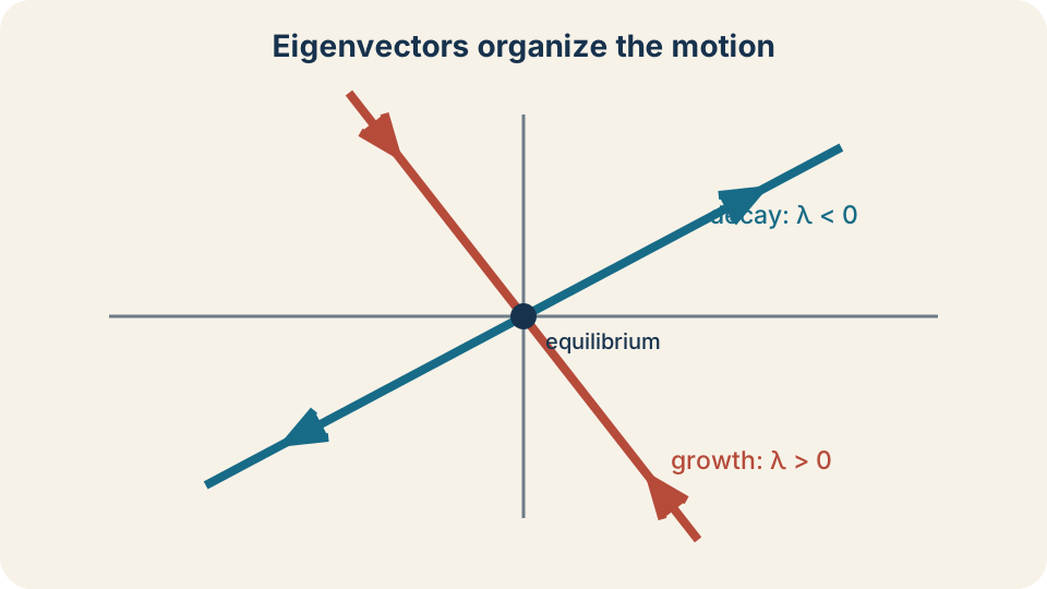
Eigenvectors identify invariant directions, while eigenvalues determine how amplitudes along those directions change.

Begin with the state and equilibrium

Consider $\mathbf{x}'=A\mathbf{x}$, where $\mathbf{x}(t)=\begin{pmatrix}x(t)\\y(t)\end{pmatrix}$ and $A=\begin{pmatrix}a&b\\c&d\end{pmatrix}$. Componentwise, the system means $x'=ax+by$ and $y'=cx+dy$. The entries $a,b,c,$ and $d$ are coupling coefficients. For example, $b$ measures how the current value of $y$ contributes to the instantaneous change of $x$. If time is measured in seconds and state components have compatible units, the matrix entries have units $\mathrm{s}^{-1}$.

An equilibrium is a state that produces no change, so it satisfies $\mathbf{x}'=\mathbf{0}$. The origin is always an equilibrium of a homogeneous linear system because $A\mathbf{0}=\mathbf{0}$. If $A$ is invertible, the origin is the only equilibrium. If $A$ is singular, a line or larger set of equilibria can occur. Standard node, saddle, and spiral classifications normally assume that the equilibrium is isolated.

Stability asks what happens after a small displacement from equilibrium. A stable equilibrium keeps sufficiently small disturbances nearby. An asymptotically stable equilibrium also draws those disturbances back as time increases. A trajectory can remain nearby without converging, as happens around an ideal center. One approaching trajectory cannot prove stability because another nearby trajectory may depart in a different direction.

Why eigenvectors are natural directions

An eigenpair $(\lambda,\mathbf{v})$ satisfies $A\mathbf{v}=\lambda\mathbf{v}$, where $\mathbf{v}\ne\mathbf{0}$. The scalar $\lambda$ is the eigenvalue, and $\mathbf{v}$ is an associated eigenvector. Multiplication by a matrix normally changes both direction and length. Multiplication of an eigenvector changes only its signed scale. Consequently, the line through an eigenvector is invariant under the differential equation.

Suppose a solution has the form $\mathbf{x}(t)=q(t)\mathbf{v}$, where $q$ is an unknown scalar amplitude. Differentiation gives $\mathbf{x}'=q'\mathbf{v}$, while substitution gives $A\mathbf{x}=qA\mathbf{v}=q\lambda\mathbf{v}$. Equating the expressions produces $q'\mathbf{v}=\lambda q\mathbf{v}$. Since $\mathbf{v}$ is nonzero, this reduces to $q'=\lambda q$. The scalar solution is $q(t)=Ce^{\lambda t}$, so $\mathbf{x}(t)=Ce^{\lambda t}\mathbf{v}$.

Every factor in this formula carries information. The constant $C$ records how much of the initial state lies in the eigenvector direction. The product $\lambda t$ must be dimensionless, so an eigenvalue has reciprocal-time units. A negative real eigenvalue makes $e^{\lambda t}$ shrink, whereas a positive one makes it grow. An imaginary component generates oscillation, which appears as rotation when two components are viewed together.

Combine independent modes

Suppose $A$ has independent real eigenvectors $\mathbf{v}_1$ and $\mathbf{v}_2$ with eigenvalues $\lambda_1$ and $\lambda_2$. Every initial state can then be written as $\mathbf{x}(0)=C_1\mathbf{v}_1+C_2\mathbf{v}_2$. Linearity allows the modal solutions to be added. The result is $\mathbf{x}(t)=C_1e^{\lambda_1t}\mathbf{v}_1+C_2e^{\lambda_2t}\mathbf{v}_2$. The constants are fixed by the initial condition rather than by the differential equation alone.

Long-term behavior is governed by modes that decay most slowly or grow most rapidly. If $\lambda_1=-1\,\mathrm{s}^{-1}$ and $\lambda_2=-4\,\mathrm{s}^{-1}$, both modes decay. However, $e^{-4t}$ becomes small much sooner than $e^{-t}$ when $t$ is measured in seconds. A generic trajectory therefore becomes nearly parallel to $\mathbf{v}_1$ late in time. The eigenvalue closest to zero is the dominant eigenvalue in this stable example.

Modal coefficients explain exceptional trajectories. If $C_1=0$, the slower mode is absent and the solution remains on the faster eigendirection. A phase portrait contains these special straight solutions as well as generic curved trajectories. Seeing one unusual curve does not overturn the overall classification. It identifies an initial condition in which one natural mode is missing.

Real eigenvalues produce nodes and saddles

When both real eigenvalues are negative, every modal exponential approaches zero as $t\to\infty$. With two independent eigenvectors, every solution is a combination of decaying modes. The origin is then an asymptotically stable node. Trajectories usually approach tangent to the eigendirection associated with the eigenvalue closest to zero. Phase-plane arrows point inward because increasing time reduces the state magnitude.

For $A=\begin{pmatrix}-1&0\\0&-3\end{pmatrix}\,\mathrm{s}^{-1}$, the solution is $x(t)=C_1e^{-t}$ and $y(t)=C_2e^{-3t}$ for time in seconds. The $y$ component decays more rapidly, so generic trajectories flatten toward the $x$-axis. The eigenvalue $-3\,\mathrm{s}^{-1}$ does not mean the state loses three units each second. It describes an instantaneous fractional rate of negative three per second. Its characteristic time is $\tau=\frac{1}{|\lambda|}=\frac{1}{3}\,\mathrm{s}$.

If both eigenvalues are positive, nonzero modal components grow and the origin is an unstable node or source. If one is positive and one is negative, the origin is a saddle. The negative-eigenvalue line attracts, while the positive-eigenvalue line repels. A saddle is unstable even though its stable eigendirection contains trajectories that approach the origin. Stability concerns every sufficiently small disturbance, not one selected path.

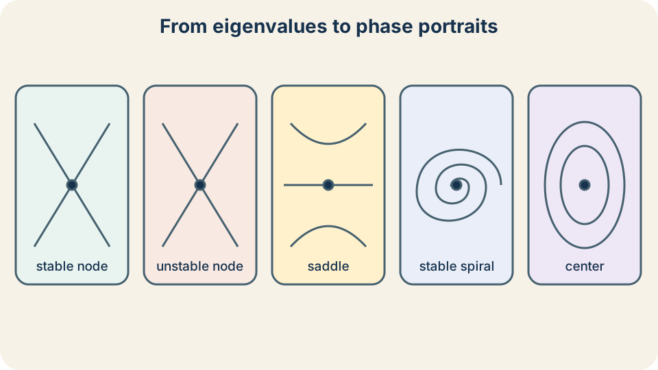
Trajectory shapes translate eigenvalue signs and imaginary parts into phase-space motion. An inward node represents two real decaying modes. A saddle combines one attracting direction with one repelling direction. A spiral combines rotation with changing amplitude. A center rotates without either exponential growth or decay. The arrows establish the direction of increasing time.

Follow a saddle from initial state to outcome

Take $A=\begin{pmatrix}1&0\\0&-2\end{pmatrix}\,\mathrm{s}^{-1}$. The eigenvalues are $1\,\mathrm{s}^{-1}$ and $-2\,\mathrm{s}^{-1}$. Their eigenvectors lie along the $x$- and $y$-axes, respectively. The general solution is $x(t)=C_1e^t$ and $y(t)=C_2e^{-2t}$ for time in seconds. These formulas display one growing amplitude and one decaying amplitude.

If $C_1=0$, the state lies on the $y$-axis and approaches the origin. If $C_2=0$, it lies on the $x$-axis and moves away. A generic state contains both components, so it may first approach while the decaying component is visible. Eventually the growing component dominates and the trajectory departs. This approach-then-depart behavior gives the saddle its familiar curved branches.

In a linear system, the stable and unstable sets are straight eigenvector lines. In a nonlinear system, corresponding curves can bend into stable and unstable manifolds. They remain tangent to the relevant eigenvectors near a hyperbolic equilibrium. These curves can divide initial conditions that lead to different outcomes. Eigenvectors therefore identify organizing structures rather than decorative lines.

Complex eigenvalues combine scaling and rotation

A real $2\times2$ matrix can have eigenvalues $\lambda=\alpha\pm i\beta$. The symbol $i$ satisfies $i^2=-1$, $\alpha$ is the real part, and $\beta$ is the imaginary magnitude. Euler’s formula states $e^{i\beta t}=\cos(\beta t)+i\sin(\beta t)$. Sine and cosine mix the state components and create rotation. The shared factor $e^{\alpha t}$ expands or contracts the rotating motion.

If $\alpha<0$, trajectories spiral inward and the equilibrium is an asymptotically stable spiral. If $\alpha>0$, they spiral outward and the equilibrium is unstable. If $\alpha=0$, the linear motion has constant amplitude and produces a center. A center is stable but not asymptotically stable because nonzero trajectories do not converge. The real part controls stability, while the imaginary part controls oscillation.

The angular frequency is $|\beta|$, and the period is $T=\frac{2\pi}{|\beta|}$. If $\beta=2\,\mathrm{rad}\,\mathrm{s}^{-1}$, then $T=\pi\,\mathrm{s}$ because radians are dimensionless here. Eigenvalues alone may not show clockwise or counterclockwise rotation. Evaluate the vector field at a convenient point such as $(1,0)$ to determine orientation. The vertical velocity there shows whether the trajectory initially moves above or below the horizontal axis.

Repeated eigenvalues require another question

A repeated eigenvalue occurs when the characteristic polynomial has one root of multiplicity two. If the matrix has two independent eigenvectors, it remains diagonalizable. The simplest case is $A=\lambda I$, where every nonzero vector is an eigenvector. All trajectories are straight rays because $\mathbf{x}(t)=e^{\lambda t}\mathbf{x}(0)$. Negative $\lambda$ yields an inward star node, while positive $\lambda$ yields an outward star node.

A repeated eigenvalue may instead have only one independent eigenvector. Such a matrix is defective, and a generalized eigenvector supplies the second solution. That solution contains a factor of $t$, often in the form $e^{\lambda t}(t\mathbf{v}+\mathbf{w})$. The polynomial factor shears trajectories toward the sole eigendirection. The sign of nonzero $\lambda$ still determines stability because exponential behavior eventually dominates polynomial behavior.

For $A=\begin{pmatrix}-2&1\\0&-2\end{pmatrix}\,\mathrm{s}^{-1}$, the repeated eigenvalue is $-2\,\mathrm{s}^{-1}$ and only one eigendirection exists. Direct solution gives $y(t)=C_2e^{-2t}$ and $x(t)=(C_1+C_2t)e^{-2t}$. Both components approach zero because $te^{-2t}\to0$ as $t\to\infty$. The origin is an asymptotically stable improper node. Counting algebraic roots without checking eigenvectors would miss that geometry.

Use trace and determinant as a reasoning map

For $A=\begin{pmatrix}a&b\\c&d\end{pmatrix}$, eigenvalues satisfy $\det(A-\lambda I)=0$. Expansion gives $\lambda^2-\tau\lambda+\Delta=0$, where $\tau=\operatorname{tr}(A)=a+d$ and $\Delta=\det(A)=ad-bc$. The quadratic formula yields $\lambda_{1,2}=\frac{\tau\pm\sqrt{\tau^2-4\Delta}}{2}$. The trace equals the eigenvalue sum. The determinant equals their product.

The discriminant $D=\tau^2-4\Delta$ determines eigenvalue type. Positive $D$ gives distinct real roots, zero $D$ gives repeated roots, and negative $D$ gives a complex-conjugate pair. If $\Delta<0$, the eigenvalue product is negative, so the equilibrium is a saddle. If $\Delta>0$, the sign of $\tau$ distinguishes attraction from repulsion. Negative trace gives negative real parts, while positive trace gives positive real parts.

Boundary cases demand care. If $\Delta=0$, at least one eigenvalue is zero and the equilibrium may not be isolated. If $\tau=0$, $\Delta>0$, and $D<0$, the roots are purely imaginary and the linear system has a center. If $D=0$, eigenvectors must be counted before the node is sketched. The trace–determinant map is a reasoning aid with meaningful boundaries rather than an infallible lookup chart.

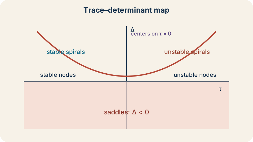
The parabola $\Delta=\frac{\tau^2}{4}$ separates real roots from complex roots, while the axes mark boundary cases. Points below the horizontal axis represent saddles because the determinant is negative. The left half of the upper region is stable because the trace is negative. The right half is unstable because the trace is positive. The vertical axis above the parabola contains linear centers and therefore requires care for nonlinear systems. Points on a boundary need more analysis than an interior point.

Work a stable node completely

Let $A=\begin{pmatrix}0&1\\-2&-3\end{pmatrix}\,\mathrm{s}^{-1}$. Its trace is $-3\,\mathrm{s}^{-1}$ and its determinant is $2\,\mathrm{s}^{-2}$. Determinant has squared reciprocal-time units because it is the product of two eigenvalues. The characteristic equation is $\lambda^2+3\lambda+2=0$. Factoring gives $(\lambda+1)(\lambda+2)=0$, so the origin is a stable node.

For $\lambda_1=-1\,\mathrm{s}^{-1}$, an eigenvector is $\mathbf{v}_1=\begin{pmatrix}1\\-1\end{pmatrix}$. For $\lambda_2=-2\,\mathrm{s}^{-1}$, an eigenvector is $\mathbf{v}_2=\begin{pmatrix}1\\-2\end{pmatrix}$. The general solution is $\mathbf{x}(t)=C_1e^{-t}\mathbf{v}_1+C_2e^{-2t}\mathbf{v}_2$ when $t$ is in seconds. Both modes decay, but the first is slower. Generic trajectories approach tangent to $\mathbf{v}_1$.

Suppose $\mathbf{x}(0)=\begin{pmatrix}3\\-4\end{pmatrix}$. Solving $C_1\mathbf{v}_1+C_2\mathbf{v}_2=\mathbf{x}(0)$ gives $C_1=2$ and $C_2=1$. Therefore $\mathbf{x}(t)=2e^{-t}\begin{pmatrix}1\\-1\end{pmatrix}+e^{-2t}\begin{pmatrix}1\\-2\end{pmatrix}$. The coefficients reveal how much of each natural mode appears initially. The classification describes the family, whereas these constants identify one member.

Distinguish a spiral from a center

Consider $A=\begin{pmatrix}0&1\\-4&-2\end{pmatrix}\,\mathrm{s}^{-1}$. Its trace is $-2\,\mathrm{s}^{-1}$ and determinant is $4\,\mathrm{s}^{-2}$. The discriminant is $-12\,\mathrm{s}^{-2}$, so the eigenvalues are complex. The quadratic formula gives $-1\pm i\sqrt{3}\,\mathrm{s}^{-1}$. The negative real part and nonzero imaginary part establish a stable spiral.

The envelope decays as $e^{-t}$ for time in seconds. The angular frequency is $\sqrt{3}\,\mathrm{rad}\,\mathrm{s}^{-1}$, so $T=\frac{2\pi}{\sqrt{3}}\,\mathrm{s}$. At $(1,0)$, the vector field is $(0,-4)$ in suitable state-units per second. The downward velocity from the positive horizontal axis establishes clockwise rotation. The state circles while its overall amplitude diminishes.

Now change the lower-right entry from $-2$ to $0$. The new matrix has trace zero, determinant $4\,\mathrm{s}^{-2}$, and eigenvalues $\pm2i\,\mathrm{s}^{-1}$. Trajectories become closed curves instead of inward spirals. The origin is a center rather than an attractor. Removing damping has changed asymptotic stability into persistent oscillation.

Linearize nonlinear systems with a Jacobian

Consider a nonlinear autonomous system $\mathbf{x}'=\mathbf{f}(\mathbf{x})$. An equilibrium $\mathbf{x}^*$ satisfies $\mathbf{f}(\mathbf{x}^*)=\mathbf{0}$. Write a nearby state as $\mathbf{x}=\mathbf{x}^*+\mathbf{u}$, where $\mathbf{u}$ is a small displacement. A first-order Taylor approximation gives $\mathbf{u}'\approx J\mathbf{u}$. Here $J=D\mathbf{f}(\mathbf{x}^*)$ is the Jacobian evaluated at the equilibrium.

For $\mathbf{f}(x,y)=\begin{pmatrix}f(x,y)\\g(x,y)\end{pmatrix}$, the Jacobian is $J=\begin{pmatrix}\frac{\partial f}{\partial x}&\frac{\partial f}{\partial y}\\\frac{\partial g}{\partial x}&\frac{\partial g}{\partial y}\end{pmatrix}$. Every partial derivative must be evaluated at $(x^*,y^*)$ before eigenvalues are computed. The matrix describes the leading response to a small displacement. Higher-order terms become relatively less important near the equilibrium. This construction bridges nonlinear dynamics and linear eigenvalue analysis.

The conclusion is local. A Jacobian near one equilibrium does not describe distant trajectories, other equilibria, or global limit cycles. A nonlinear system can contain several equilibria with different classifications. Its phase portrait can include barriers and attracting sets that no single local matrix predicts. Eigenvalue stability is powerful precisely because its scope is stated clearly.

Know when linearization is decisive

An equilibrium is hyperbolic when no Jacobian eigenvalue has zero real part. Nodes, saddles, and inward or outward spirals are hyperbolic when their defining real parts are strictly nonzero. Near such an equilibrium, the nonlinear portrait has the same essential local structure as its linearization. Curves may bend and speeds may change, but attraction, repulsion, and saddle structure persist. This robustness justifies transferring the classification locally.

Suppose a Jacobian has eigenvalues $-2\,\mathrm{s}^{-1}$ and $-0.1\,\mathrm{s}^{-1}$. Both real parts are negative, so the nonlinear equilibrium is locally asymptotically stable. The smaller magnitude identifies a slow direction that dominates late transients. Nonlinear terms can alter exact paths and the size of the attracting neighborhood. They do not reverse the classification sufficiently close to this hyperbolic equilibrium.

If any eigenvalue has zero real part, linearization may be inconclusive. The equations $x'=x^3$ and $x'=-x^3$ both linearize to $u'=0$ at the origin. Nevertheless, the first origin is unstable and the second is asymptotically stable. Higher-order terms decide the behavior because the linear rate vanishes. Purely imaginary Jacobian eigenvalues likewise do not automatically prove that a nonlinear equilibrium is a center.

Follow a reliable classification workflow

First locate every equilibrium and form the correct matrix. Use $A$ directly for a homogeneous linear system. For a nonlinear system, solve $\mathbf{f}(\mathbf{x}^*)=\mathbf{0}$ and evaluate a separate Jacobian at each solution. Then compute trace, determinant, and discriminant in two dimensions. Find eigenvectors when a phase portrait or explicit solution is required.

Next translate the spectrum into motion. Negative real parts mean decay, positive real parts mean growth, opposite signs mean a saddle, and nonzero imaginary parts mean oscillation. Check one vector-field arrow to determine rotational direction. For repeated roots, count independent eigenvectors. For nonlinear systems, verify hyperbolicity before transferring the classification.

Finally test the interpretation against units, geometry, and initial conditions. Eigenvalues require reciprocal-time units, and exponential arguments must be dimensionless. Identify the dominant mode and exceptional trajectories with a zero modal coefficient. State whether the result is global for a linear system or local for a nonlinear one. A classification is complete only when calculation and language agree.

Repair common mistakes

One mistake is to use $|\lambda|$ rather than $\operatorname{Re}(\lambda)$ to judge stability. Complex values with equal magnitudes can have opposite real parts and opposite stability. Write each eigenvalue as $\alpha+i\beta$ and inspect $\alpha$ first. Another mistake is to claim that an imaginary part causes instability. Imaginary parts create oscillation, whereas real parts control exponential growth or decay.

A second mistake is to call a saddle stable because one observed trajectory approaches the origin. Saddles contain a stable direction, but nearby states off that direction eventually depart. Ask whether every sufficiently small displacement remains small. One positive real part makes the answer no. Stability is a neighborhood property rather than a property of one trajectory.

A third mistake is to transfer a center from a Jacobian automatically to a nonlinear system. Purely imaginary eigenvalues make the equilibrium nonhyperbolic. Higher-order terms or conserved quantities must then be examined. Zero trace or zero determinant should likewise trigger a boundary analysis instead of a memorized label. Precise qualification is part of mathematical rigor.

Practice, retrieve, and synthesize

Suppose a matrix has trace $-5\,\mathrm{s}^{-1}$ and determinant $6\,\mathrm{s}^{-2}$. The discriminant is $1\,\mathrm{s}^{-2}$, so the eigenvalues are distinct and real. Their positive product and negative sum imply that both are negative. The origin is therefore an asymptotically stable node. Direct calculation gives $-2\,\mathrm{s}^{-1}$ and $-3\,\mathrm{s}^{-1}$.

Now suppose the trace is $2\,\mathrm{min}^{-1}$ and determinant is $5\,\mathrm{min}^{-2}$. The discriminant is $-16\,\mathrm{min}^{-2}$, giving $1\pm2i\,\mathrm{min}^{-1}$. The positive real part makes the equilibrium unstable. The imaginary part makes trajectories rotate, so it is an unstable spiral. A vector-field sample is still needed to determine its orientation.

Eigenvectors identify invariant state patterns, and eigenvalues attach growth, decay, and oscillation to those patterns. Trace, determinant, and discriminant summarize the same information efficiently in two dimensions. Hyperbolic Jacobians transfer that classification to nearby nonlinear motion, while zero real parts demand further analysis. The next step is to compare these predictions with nullclines and numerical trajectories. Understanding is demonstrated when every sign, unit, direction, and qualification can be explained rather than merely named.