Characteristic Roots Classify Linear ODE Solutions

A characteristic equation translates a constant-coefficient differential equation into an algebraic polynomial. That translation is powerful because polynomial roots encode whether solutions grow, decay, oscillate, or combine those behaviors. The method is not a magic substitution pulled from nowhere. It works because exponential functions retain their basic form under repeated differentiation. Understanding that mechanism makes the root cases easier to reconstruct and interpret.

The problem the method solves

Consider a second-order homogeneous linear equation $ay''+by'+cy=0$. The coefficients $a$, $b$, and $c$ are constants, and $a\neq0$ so the equation is genuinely second order. The unknown function is $y(t)$, where $t$ may represent time or another independent variable. The primes indicate derivatives with respect to $t$. Homogeneous means the right side is zero.

The method applies directly because the coefficients do not change with $t$. A variable-coefficient equation such as $t^2y''+ty'-y=0$ requires different reasoning even though its appearance is similar. A nonhomogeneous equation such as $ay''+by'+cy=f(t)$ also requires a particular solution in addition to the homogeneous response. The characteristic roots still describe its complementary homogeneous part. Scope must be identified before calculation begins.

A second-order equation generally needs two independent solution functions. Their linear combination contains two constants that can be set by two independent conditions. Common initial conditions are $y(0)=y_0$ and $y'(0)=v_0$. The symbol $y_0$ is the initial function value, while $v_0$ is its initial rate of change. The characteristic method must therefore produce a two-dimensional solution space.

Why exponentials are the natural trial functions

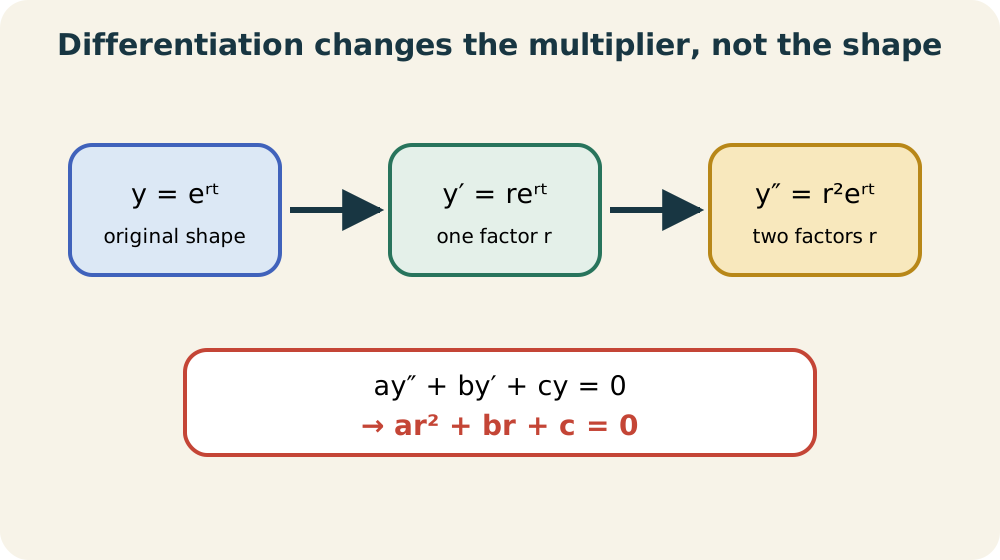
Suppose $y=e^{rt}$, where $r$ is a constant to be determined. Differentiation gives $y'=re^{rt}$ and $y''=r^2e^{rt}$. Each derivative is the original exponential multiplied by a power of $r$. The function’s shape does not change under differentiation. This property lets all three differential terms share a common factor.

Substitution produces $a(r^2e^{rt})+b(re^{rt})+ce^{rt}=0$. Factoring gives $(ar^2+br+c)e^{rt}=0$. The exponential $e^{rt}$ is never zero for real $t$, even when $r$ is complex. Therefore the polynomial factor must equal zero. The characteristic equation is $ar^2+br+c=0$.

The trial function is connected to an eigenfunction idea. The differentiation operator sends $e^{rt}$ to the same function multiplied by $r$. Applying a polynomial in the derivative operator sends it to the same function multiplied by the corresponding polynomial in $r$. A root makes that multiplier zero. The differential problem has thereby become an algebraic condition on possible exponential rates.

Constructing the polynomial carefully

The characteristic polynomial mirrors derivative order. A term $ay''$ becomes $ar^2$, a term $by'$ becomes $br$, and a term $cy$ becomes $c$. Missing derivative orders produce zero coefficients rather than disappearing conceptually. For example, $y''-9y=0$ gives $r^2-9=0$. The absent $y'$ term corresponds to coefficient zero.

Signs must be copied exactly. The equation $y''-4y'+3y=0$ gives $r^2-4r+3=0$, not $r^2+4r+3=0$. It factors as $(r-1)(r-3)=0$. The roots are $r=1$ and $r=3$. Both positive roots anticipate exponential growth.

If the leading coefficient is not one, it remains in the polynomial. The equation $2y''+5y'-3y=0$ gives $2r^2+5r-3=0$. Factoring gives $(2r-1)(r+3)=0$, so the roots are $\frac{1}{2}$ and $-3$. Dividing the original ODE by two first would give the same roots. Scaling the entire equation by a nonzero constant does not change its solution set.

Roots are behavior labels

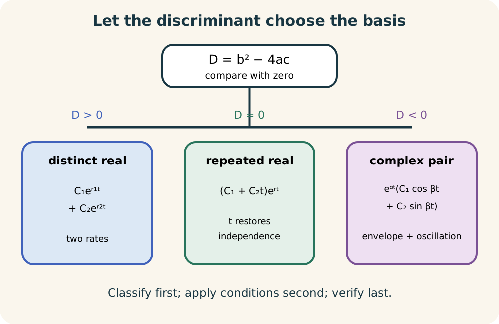
The quadratic formula gives $r=\frac{-b\pm\sqrt{b^2-4ac}}{2a}$. The discriminant $D=b^2-4ac$ classifies the root pattern. When $D>0$, there are two distinct real roots. When $D=0$, there is one repeated real root. When $D<0$, the roots form a complex-conjugate pair.

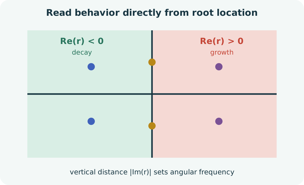
The sign and type of each root predict qualitative behavior before initial conditions are applied. A positive real part produces exponential growth, while a negative real part produces exponential decay. A zero real part produces neither exponential growth nor decay. A nonzero imaginary part produces oscillation. Initial conditions determine the mixture and amplitude but do not change the available fundamental behaviors.

This separation between structure and state is pedagogically valuable. Coefficients determine the roots, and roots determine the basis of the solution space. Initial conditions choose one trajectory from that space. A model parameter change can alter the root pattern itself. An initial-state change cannot turn real roots into complex roots because it does not change the equation.

Distinct real roots

If the characteristic roots are distinct real numbers $r_1$ and $r_2$, the general solution is $y=C_1e^{r_1t}+C_2e^{r_2t}$. The constants $C_1$ and $C_2$ are determined by conditions. Each exponential separately satisfies the ODE because its rate is a root. Linearity allows their sum to satisfy the homogeneous equation. Distinct exponential rates are linearly independent.

Consider $y''-y'-6y=0$. Its characteristic polynomial is $r^2-r-6=(r-3)(r+2)$. The roots are $3$ and $-2$, giving $y=C_1e^{3t}+C_2e^{-2t}$. One mode grows while the other decays. Unless initial conditions make $C_1=0$, the growing mode eventually dominates as $t$ increases.

Dominance does not mean the smaller mode is absent at finite times. Near the initial time, both constants can strongly affect the shape. For negative time, the mode that decays forward can grow backward. Statements about long-term behavior must specify the direction of time. A qualitative classification should name roots, modes, and any exceptional initial-condition cancellation.

Applying two initial conditions

Use the previous solution $y=C_1e^{3t}+C_2e^{-2t}$ with $y(0)=4$ and $y'(0)=1$. At $t=0$, both exponentials equal one, so $C_1+C_2=4$. Differentiation gives $y'=3C_1e^{3t}-2C_2e^{-2t}$. The second condition gives $3C_1-2C_2=1$. These two linear equations determine the two constants.

Solving yields $C_1=\frac{9}{5}$ and $C_2=\frac{11}{5}$. Therefore $y=\frac{9}{5}e^{3t}+\frac{11}{5}e^{-2t}$. Substitution at $t=0$ verifies $y(0)=\frac{20}{5}=4$. Differentiating and substituting verifies $y'(0)=\frac{27}{5}-\frac{22}{5}=1$. Both checks are required because a second-order solution must satisfy both conditions.

The coefficient of the growing mode is nonzero, so long-term growth is expected. Its initial contribution is smaller than the decaying contribution, but exponential rate eventually matters more than starting coefficient. This example separates exact solution from behavior interpretation. The constants describe the selected state, while the roots describe modes available to every solution. A complete answer should include both layers.

Repeated roots require a second solution

If the polynomial has a repeated root $r$, one solution is $e^{rt}$. Writing the same function twice does not create two independent solutions. A second-order equation still needs a second independent function. The required companion is $te^{rt}$. Thus the general repeated-root solution is $y=(C_1+C_2t)e^{rt}$.

The factor $t$ can be understood in several ways. It arises through reduction of order, through a limiting process as two distinct roots approach one another, or through generalized eigenvector structure in a first-order system. At a foundational level, direct substitution verifies that $te^{rt}$ works when the root is repeated. Its presence is not an arbitrary decoration. It restores the missing independent direction in the solution space.

Consider $y''+6y'+9y=0$. The polynomial is $(r+3)^2$, so $r=-3$ is repeated. The solution is $y=(C_1+C_2t)e^{-3t}$. Both basis functions decay as $t$ grows, although the $t$ factor can create a temporary turn. There is no sinusoidal oscillation because the roots have no imaginary part.

Repeated-root initial-value example

Apply $y(0)=2$ and $y'(0)=0$ to $y=(C_1+C_2t)e^{-3t}$. The first condition gives $C_1=2$. Differentiate using the product rule to obtain $y'=[C_2-3(C_1+C_2t)]e^{-3t}$. At $t=0$, the derivative condition becomes $C_2-3C_1=0$. Therefore $C_2=6$.

The solution is $y=(2+6t)e^{-3t}$. At the initial instant, the increasing linear factor exactly balances the decreasing exponential in the derivative. Afterward, the exponential dominates and the solution approaches zero. It may initially change curvature without crossing back and forth periodically. A graph should be interpreted through both factors.

Repeated negative roots often appear at the critical boundary between oscillatory and nonoscillatory response in physical systems. In a damped oscillator, this is associated with critical damping. The mathematical term $te^{rt}$ reflects degeneracy of the two exponential modes. The physical interpretation depends on the coefficients and modeled quantities. Algebraic classification and physical explanation should support each other without being conflated.

Complex roots produce real oscillations

When $D<0$, the roots are $r=\alpha\pm i\beta$. The symbol $i$ satisfies $i^2=-1$, $\alpha$ is the real part, and $\beta$ is the magnitude of the imaginary part. Complex exponential solutions are $e^{(\alpha+i\beta)t}$ and $e^{(\alpha-i\beta)t}$. Euler’s identity connects them to real sine and cosine functions. Real-coefficient ODEs therefore have a real-valued basis.

The real general solution is $y=e^{\alpha t}(C_1\cos\beta t+C_2\sin\beta t)$. The exponential envelope $e^{\alpha t}$ controls amplitude growth or decay. The trigonometric factors produce oscillation with angular frequency $|\beta|$. The period is $T=\frac{2\pi}{|\beta|}$ when $\beta\neq0$. Constants choose phase and amplitude according to initial conditions.

Three qualitative cases follow immediately. If $\alpha<0$, the oscillation decays. If $\alpha=0$, the ideal oscillation maintains constant amplitude. If $\alpha>0$, oscillation grows. A complex root does not mean the physical quantity itself must be imaginary. The conjugate pair combines into a real response.

Complex-root worked example

Solve $y''-2y'+5y=0$. The characteristic equation is $r^2-2r+5=0$. Applying the quadratic formula gives $r=1\pm2i$. Therefore $\alpha=1$ and $\beta=2$. The general solution is $y=e^t(C_1\cos2t+C_2\sin2t)$.

Before applying conditions, interpret the roots. The real part $1$ produces an envelope that grows as $e^t$. The imaginary magnitude $2$ gives angular frequency $2$ radians per unit time. The period is $T=\frac{2\pi}{2}=\pi$ time units. The equation describes a growing oscillation.

Suppose $y(0)=3$ and $y'(0)=1$. The first condition gives $C_1=3$. Differentiating and evaluating at zero gives $y'(0)=C_1+2C_2=1$. Thus $C_2=-1$, and $y=e^t(3\cos2t-\sin2t)$. Substitution into both initial conditions checks the constants.

A discriminant-to-solution workflow

Begin by placing the ODE in homogeneous constant-coefficient standard form. Confirm that the coefficient of the highest derivative is nonzero. Replace each derivative order with the corresponding power of $r$. Solve the resulting polynomial exactly when possible. Keep complex roots in $\alpha\pm i\beta$ form for interpretation.

Next select the solution template from root multiplicity and type. Distinct real roots require two exponentials, a repeated root requires the $t$ multiplier, and complex roots require a sine-cosine pair with an exponential envelope. Do not apply initial conditions before the correct general form has been built. Differentiate that form carefully. Solve the resulting algebraic system for constants.

Finally verify and interpret. Substitute the solution or its basis functions into the original ODE. Check every initial or boundary condition. Describe growth, decay, oscillation, frequency, and long-term dominance using root information. This workflow separates classification errors from algebra errors and makes debugging easier.

Higher-order equations

The same method extends to higher-order homogeneous linear ODEs with constant coefficients. An $n$th-order equation produces a degree-$n$ characteristic polynomial. Counting multiplicity over the complex numbers gives $n$ roots. Those roots generate $n$ independent basis functions when repeated-root factors are handled properly. The solution space has dimension $n$.

If a real root $r$ has multiplicity $m$, its contributions are $e^{rt},te^{rt},\ldots,t^{m-1}e^{rt}$. The ellipsis indicates all integer powers through $m-1$. A complex-conjugate pair with multiplicity produces analogous sine-cosine terms multiplied by successive powers of $t$. Multiplicity therefore records how many generalized modes belong to the same rate. The rule generalizes the repeated-root second-order case.

For example, $(r+1)^3=0$ produces $e^{-t}$, $te^{-t}$, and $t^2e^{-t}$. A third-order equation needs three independent constants. Although every basis function decays forward in time, polynomial factors can shape substantial transients. Long-term exponential rate still dominates powers of $t$. Root multiplicity affects form without changing the sign of the exponential rate.

Relation to first-order systems and stability

A second-order scalar ODE can be rewritten as a first-order system by defining $x_1=y$ and $x_2=y'$. The state vector contains the function value and its first derivative. The system matrix has eigenvalues equal to the characteristic roots of the scalar equation. Thus characteristic-root analysis is a special case of eigenvalue analysis. This connection unifies differential equations and linear algebra.

In a linear autonomous system, eigenvalue real parts govern local exponential growth or decay. Negative real parts correspond to asymptotic decay of all modes. A positive real part creates an unstable growing direction. Purely imaginary roots can produce neutral oscillation in the ideal linear model. Repeated or zero-real-part cases may require additional analysis because multiplicity and nonlinear effects matter.

The root plane offers a visual stability map. Left-half-plane roots decay, right-half-plane roots grow, and off-axis imaginary parts create rotation or oscillation. Moving model parameters can move roots across these boundaries. Damping, feedback, and stiffness changes can therefore alter qualitative behavior. Root locations translate algebra into a design and interpretation language.

What characteristic roots do not do

The characteristic method does not directly solve arbitrary variable-coefficient equations. Exponential functions no longer factor out with a constant polynomial when coefficients depend on $t$. Some special variable-coefficient equations admit related substitutions, but their logic must be derived separately. Pattern matching is not a substitute for checking assumptions. The phrase constant coefficient should appear explicitly in the method’s scope.

For nonhomogeneous equations, roots supply only the complementary solution. A particular solution must account for the forcing term. If the forcing duplicates a homogeneous mode, the trial particular form must be multiplied by a sufficient power of $t$. This resonance-like adjustment is connected to root multiplicity. The complete solution is complementary plus particular.

Characteristic roots also do not determine constants without conditions. They classify available modes, not the selected trajectory. An unstable mode can be absent under exactly tuned initial conditions, though perturbations may activate it. A stable equation can show a temporary increase because modes combine. Qualitative statements should distinguish generic long-term behavior from every possible short-term path.

Common mistakes and repairs

One mistake is losing signs while building the polynomial. Repair it by mapping each ODE term to one polynomial term before factoring. Another mistake is writing only $C_1e^{rt}+C_2e^{rt}$ for a repeated root. Those terms are dependent and collapse into one constant. Replace the second with $C_2te^{rt}$.

A second mistake leaves complex exponential solutions without converting them for a real-valued problem. Write roots as $\alpha\pm i\beta$ and use the real sine-cosine form. Do not confuse $\beta$ with ordinary frequency in cycles per unit time. It is angular frequency, so divide by $2\pi$ for ordinary frequency. Include the exponential envelope controlled by $\alpha$.

A third mistake applies conditions to an incomplete general solution. Classify roots and write every independent basis function first. Then differentiate the complete expression and solve for all constants. Verify both the ODE and the conditions afterward. A failed check identifies that the work is not finished even if the formula looks familiar.

Practice and retrieval

Classify the roots and write the general solution for $y''+5y'+6y=0$. Predict long-term behavior before using any initial conditions. Then apply $y(0)=1$ and $y'(0)=0$. Verify the constants by substitution at the initial time. State which mode dominates for large positive $t$.

Repeat the classification for $y''+4y'+4y=0$. Explain why two copies of $e^{-2t}$ do not form a valid basis. Write the repeated-root form and describe whether generic solutions oscillate. Identify the role of the factor $t$. Connect the root to critical-boundary behavior without claiming every such equation is a mechanical oscillator.

Finally analyze $y''+4y=0$ without solving for constants. State the characteristic roots, envelope behavior, angular frequency, and period. Explain why the complex roots still produce real solutions. Describe how the answer changes if the equation becomes $y''-4y=0$. This comparison isolates the meaning of the sign on the constant term.

Solutions and reasoning

For $y''+5y'+6y=0$, the polynomial factors as $(r+2)(r+3)$. The solution is $y=C_1e^{-2t}+C_2e^{-3t}$. Conditions give $C_1+C_2=1$ and $-2C_1-3C_2=0$, so $C_1=3$ and $C_2=-2$. Thus $y=3e^{-2t}-2e^{-3t}$. The $e^{-2t}$ mode decays more slowly and dominates generically.

For $y''+4y'+4y=0$, the polynomial is $(r+2)^2$. The basis is $e^{-2t}$ and $te^{-2t}$, not two identical exponentials. The general solution is $(C_1+C_2t)e^{-2t}$. Generic solutions decay without sinusoidal oscillation. The $t$ factor supplies the independent companion required by multiplicity.

For $y''+4y=0$, roots are $\pm2i$. The real part is zero, angular frequency is $2$, and period is $\pi$. Conjugate exponentials combine into $C_1\cos2t+C_2\sin2t$. Changing the sign gives roots $\pm2$ and solution $C_1e^{2t}+C_2e^{-2t}$. The behavior changes from neutral oscillation to competing growth and decay.

Connection forward

Characteristic roots provide the homogeneous backbone for forced differential equations. Particular-solution methods add the response created by an external input. When forcing matches a homogeneous mode, resonance and trial-form adjustment appear. The same roots still control transients and stability. This separation is central in vibration, circuit, and control models.

The method also prepares the transition to systems of equations. Matrix eigenvalues replace scalar polynomial roots, while eigenvectors determine state-space directions. Complex eigenvalues generate spiral or rotational behavior, and repeated eigenvalues raise questions about diagonalizability. The scalar examples offer a concrete foundation for those ideas. Linear algebra then reveals why the patterns generalize.

Carry forward a compact interpretive statement. The characteristic polynomial encodes the differential operator’s exponential modes. Root real parts control growth or decay, imaginary parts control oscillation, and multiplicity controls the necessary polynomial factors. Initial conditions choose a combination of those modes. With that statement understood, the formulas can be rebuilt instead of merely recalled.