Second-Order ODEs Govern Oscillation and Motion

Acceleration is a second derivative, so laws connecting force and motion naturally create second-order differential equations. The same mathematical structure describes a suspended mass, a small-angle pendulum, an electrical circuit, a vibrating building, and many feedback systems. These models differ physically, but each balances inertia-like behavior, resistance, restoration, and external input. Their solutions reveal whether disturbances decay, persist, oscillate, or grow. Understanding that structure is more valuable than memorizing a collection of solution forms.

Begin with order, linearity, and the unknown function

A second-order ordinary differential equation contains a second derivative of an unknown function and no derivative of higher order. If the unknown is $y(t)$, then $y'$, also written $\frac{dy}{dt}$, is its first derivative and $y''$, also written $\frac{d^2y}{dt^2}$, is its second derivative. The independent variable is often time $t$, but it could be position or another scalar variable. The word ordinary means there is only one independent variable. Order describes the highest derivative present, not the highest power of the unknown.

A linear second-order equation has the form $a(t)y''+b(t)y'+c(t)y=g(t)$, where the coefficient functions depend only on $t$. The unknown $y$ and its derivatives appear only to the first power and are not multiplied together. An equation such as $y''+t^2y'+e^ty=\sin t$ is linear despite its complicated coefficients. In contrast, $y''+y^2=0$ and $yy''+(y')^2=0$ are nonlinear. The distinction matters because superposition applies only to linear equations.

The equation is homogeneous when the forcing term is zero, giving $a(t)y''+b(t)y'+c(t)y=0$. It is nonhomogeneous when $g(t)$ is not identically zero. Homogeneous does not mean that the solution itself is zero, although the zero function is always one solution. The homogeneous solution describes the system’s internal modes and initial-condition freedom. A particular solution accounts for one response to the external forcing.

Explain why two initial conditions are needed

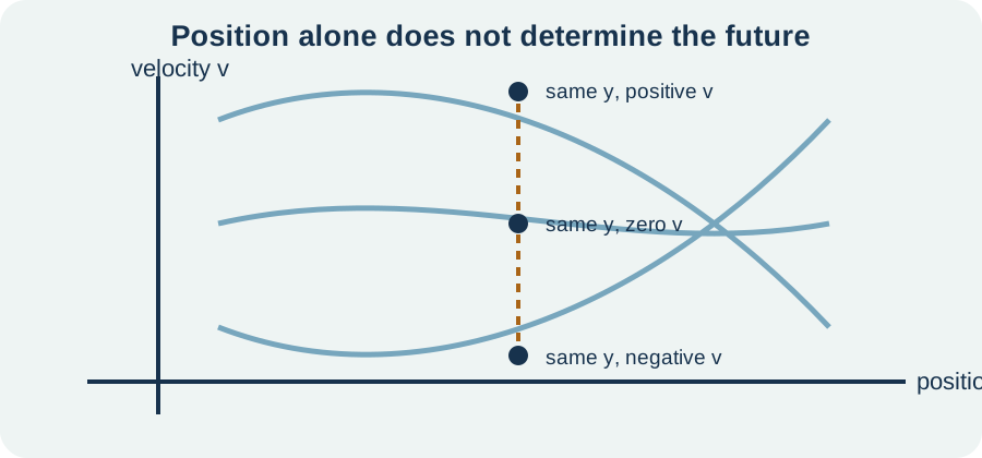
Solving a second-order equation generally introduces two independent constants. Two scalar conditions are therefore needed to select one member from the solution family. For a motion problem, these are commonly position $y(t_0)=y_0$ and velocity $y'(t_0)=v_0$. Position alone does not reveal whether the object is moving left, moving right, or momentarily at rest. Different velocities can produce different futures through the same position.

Geometrically, rewrite the equation as a first-order system by setting $v=y'$. Then $y'=v$ and $v'$ is determined by the original equation. The state is the ordered pair $(y,v)$ rather than position alone. One initial position and one initial velocity specify one point in this two-dimensional phase space. Under suitable existence and uniqueness conditions, that state determines one local trajectory.

Other pairs of conditions may determine a solution, but they require analysis. Boundary-value problems may specify $y$ at two different independent-variable values rather than specifying $y$ and $y'$ at one point. Such conditions can yield one solution, many solutions, or no solution depending on the equation and values. Initial-value and boundary-value problems should not be treated as interchangeable. The location and type of each condition matter.

Connect the equation to force balance

For a mass moving along one axis, Newton’s second law states that net force equals mass times acceleration. If displacement from equilibrium is $x(t)$, velocity is $x'(t)$ and acceleration is $x''(t)$. A linear spring exerts restoring force $-kx$, where stiffness $k$ is positive and the negative sign points toward equilibrium. A viscous damper exerts force $-cx'$, where damping coefficient $c$ is positive. An external force is represented by $F(t)$.

Adding the forces gives $mx''=-cx'-kx+F(t)$. Rearrangement produces the standard mass–spring–damper equation $mx''+cx'+kx=F(t)$. Each term has units of force. With SI units, $m$ is in kilograms, $x''$ is in the horizontal fraction $\frac{\mathrm m}{\mathrm s^2}$, and their product is the newton $\mathrm N$. The rearranged form places internal responses on the left and external input on the right.

Dimensional consistency determines the coefficient units. Because $x'$ has units $\frac{\mathrm m}{\mathrm s}$, the damping coefficient has units $\frac{\mathrm{N\,s}}{\mathrm m}$. Because $x$ has units of meters, stiffness has units $\frac{\mathrm N}{\mathrm m}$. Then $cx'$ and $kx$ both have units of newtons. A model whose terms do not share units cannot represent a valid force balance.

Solve constant-coefficient homogeneous equations

Consider $ay''+by'+cy=0$, where $a$, $b$, and $c$ are constants and $a\ne0$. Exponential functions are natural trial solutions because differentiating $e^{rt}$ only multiplies it by $r$. Substituting $y=e^{rt}$ gives $ar^2e^{rt}+bre^{rt}+ce^{rt}=0$. Because $e^{rt}$ is never zero, divide it out. The remaining polynomial equation $ar^2+br+c=0$ is the characteristic equation.

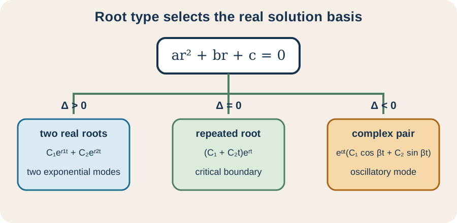
The variable $r$ is a candidate exponential growth rate, not the independent variable. Each root generates a mode compatible with the differential equation. A second-order characteristic polynomial has two roots when multiplicity and complex values are counted. Their types determine the real solution form. Initial conditions then choose the coefficients multiplying those modes.

The characteristic method applies directly to linear homogeneous equations with constant coefficients. It does not justify replacing variable coefficients with constants or applying a quadratic formula to nonlinear equations. Always classify the equation before selecting a method. A correct algebraic procedure used outside its assumptions is still incorrect. Method choice begins with structure.

Interpret distinct real roots

If the characteristic equation has distinct real roots $r_1$ and $r_2$, the general solution is $y=C_1e^{r_1t}+C_2e^{r_2t}$. The constants $C_1$ and $C_2$ are determined by conditions and are not the same as physical coefficients in the differential equation. Each exponential mode evolves independently. Linearity allows their weighted sum. Distinct roots produce independent solution functions.

If both roots are negative, both modes decay as time increases and the zero solution is asymptotically stable. If one root is positive, a generic solution contains a growing mode and moves away from zero. If one root is zero, a constant mode remains. The root with the largest real part usually dominates long-term behavior. Initial conditions can eliminate a mode only when its coefficient happens to be zero.

Solve $y''+3y'+2y=0$ by factoring $r^2+3r+2=(r+1)(r+2)$. The roots are $-1$ and $-2$, giving $y=C_1e^{-t}+C_2e^{-2t}$. Both terms decay, but $e^{-t}$ decays more slowly and usually controls the long-time response. Substitution into the original equation verifies each mode and therefore their linear combination. Initial conditions would determine the numerical constants.

Understand repeated roots

If the characteristic equation has a repeated real root $r$, one exponential $e^{rt}$ is not enough to provide two independent solution directions. A second solution is $te^{rt}$. The general solution becomes $y=(C_1+C_2t)e^{rt}$. Multiplication by $t$ creates the missing independent behavior. The repeated algebraic root therefore changes the form of the solution space.

For $y''+2y'+y=0$, the characteristic equation is $(r+1)^2=0$. The repeated root is $r=-1$, so $y=(C_1+C_2t)e^{-t}$. Both components decay as $t$ grows, even though the factor $t$ initially increases. Exponential decay ultimately dominates polynomial growth. The response returns to equilibrium without sustained oscillation.

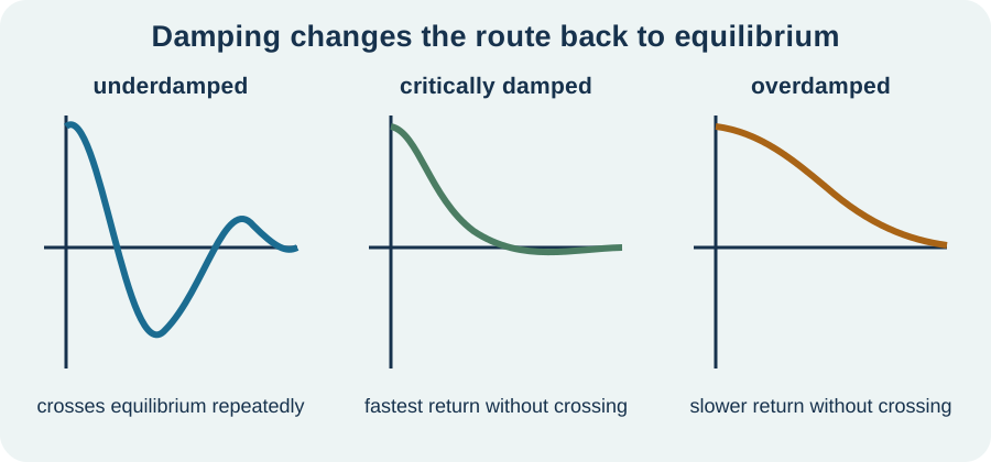
Repeated roots occur at a boundary between two distinct real roots and a complex-conjugate pair. In a mass–spring–damper model, this boundary corresponds to critical damping. It produces the fastest nonoscillatory return under the ideal linear model. The word “critical” describes a threshold, not danger. Parameter uncertainty can move a real system to either side of that boundary.

Convert complex roots into real oscillations

If the roots are $r=\alpha\pm i\beta$, where $i^2=-1$ and $\beta\ne0$, a real solution is $y=e^{\alpha t}(C_1\cos\beta t+C_2\sin\beta t)$. The real part $\alpha$ controls exponential growth or decay. The imaginary magnitude $|\beta|$ controls angular frequency. Sine and cosine appear through Euler’s relation between complex exponentials and circular oscillation. Real coefficients produce conjugate roots, allowing a real-valued solution basis.

The oscillation period is $T=\frac{2\pi}{|\beta|}$ when $t$ is time. The horizontal fraction means one full angular cycle $2\pi$ radians is divided by angular speed $|\beta|$ in radians per unit time. If $alpha<0$, the exponential envelope decays. If $alpha=0$, the amplitude remains constant in the ideal model. If $alpha>0$, oscillation grows and indicates instability.

For $y''+4y=0$, the characteristic equation $r^2+4=0$ gives $r=\pm2i$. Thus $y=C_1\cos2t+C_2\sin2t$. Its angular frequency is $2\ \frac{\mathrm{rad}}{\mathrm s}$ when $t$ is in seconds, and its period is $\pi\ \mathrm s$. The absence of damping preserves amplitude indefinitely in the mathematical model. Real systems often contain energy losses omitted by this equation.

Classify damping through the discriminant

For the unforced equation $mx''+cx'+kx=0$, the characteristic polynomial is $mr^2+cr+k$. Its discriminant is $\Delta=c^2-4mk$. The sign of $\Delta$ determines whether roots are distinct real, repeated real, or complex conjugates. Because $m$, $c$, and $k$ have physical meaning, this algebraic classification becomes a prediction about motion. Roots convert parameter balance into observable behavior.

When $c^2>4mk$, the system is overdamped and has two negative real roots for positive parameters. It returns without oscillating, but the slow mode can make the return sluggish. When $c^2=4mk$, the system is critically damped and has a repeated negative root. When $c^2<4mk$, the system is underdamped and has complex roots with negative real part. The resulting oscillations decay within an exponential envelope.

The undamped natural angular frequency is $\omega_n=\sqrt{\frac{k}{m}}$. The damping ratio is $\zeta=\frac{c}{2\sqrt{mk}}$, a dimensionless comparison of actual damping with critical damping. Values $0<\zeta<1$, $\zeta=1$, and $\zeta>1$ correspond to underdamping, critical damping, and overdamping. Dimensionless parameters make comparisons across differently scaled systems possible. They do not remove the need to report original physical coefficients.

Apply initial conditions without confusing constants

After finding the general solution, differentiate it before substituting initial velocity data. For $y=C_1e^{r_1t}+C_2e^{r_2t}$, the derivative is $y'=r_1C_1e^{r_1t}+r_2C_2e^{r_2t}$. Evaluating $y(t_0)$ and $y'(t_0)$ produces two algebraic equations for $C_1$ and $C_2$. Solve that system and substitute the constants back. Then verify both initial conditions explicitly.

The symbols used for integration constants should not duplicate physical parameters. In $mx''+cx'+kx=0$, the letter $c$ already denotes damping. Writing solution constants as $C_1$ and $C_2$ reduces ambiguity. Capitalization alone can still be overlooked, so sentences should identify each role. Clear notation matters especially when formulas are viewed on small screens.

For $y''+4y=0$ with $y(0)=3\ \mathrm m$ and $y'(0)=-2\ \frac{\mathrm m}{\mathrm s}$, begin with $y=C_1\cos2t+C_2\sin2t$. Position gives $C_1=3\ \mathrm m$. Differentiation gives $y'=-2C_1\sin2t+2C_2\cos2t$, so velocity at zero gives $2C_2=-2\ \frac{\mathrm m}{\mathrm s}$. Because the factor two has units $\frac{1}{\mathrm s}$, $C_2=-1\ \mathrm m$, and the solution is $y=3\cos2t-\sin2t$ meters. Direct evaluation at zero confirms both stated initial values.

Use superposition for forced equations

For a linear operator $L$, a nonhomogeneous equation can be written $L[y]=g(t)$. If $y_h$ satisfies $L[y_h]=0$ and $y_p$ satisfies $L[y_p]=g(t)$, then $y=y_h+y_p$ satisfies the forced equation. The homogeneous part carries two degrees of initial-condition freedom. The particular part is one selected response to the forcing. Their sum is the complete solution.

Suppose $y''+y=2$. The homogeneous solution is $y_h=C_1\cos t+C_2\sin t$. A constant trial $y_p=A$ gives $0+A=2$, so $A=2$. Therefore $y=C_1\cos t+C_2\sin t+2$. The forcing shifts the equilibrium around which the homogeneous oscillation occurs.

With $y(0)=0$ and $y'(0)=0$, position gives $C_1+2=0$ and velocity gives $C_2=0$. The solution is $y=2-2\cos t$. The constant particular response is steady, but the undamped homogeneous response does not decay. Calling one part transient would be misleading here because it persists indefinitely. The terminology must follow the actual long-time behavior.

Choose a particular-solution method deliberately

Undetermined coefficients works when constant-coefficient equations are forced by combinations of polynomials, exponentials, sines, and cosines. Choose a trial family closed under differentiation and substitute it into the equation. If the trial duplicates a homogeneous solution, multiply it by a sufficient power of $t$ to restore independence. This adjustment is sometimes called the resonance rule. Coefficients are determined by matching like terms.

Variation of parameters applies more broadly when a fundamental pair of homogeneous solutions is known. It replaces constant coefficients with functions and derives equations for those functions. The method is more flexible but algebraically heavier. Transform methods, numerical solvers, and Green’s functions provide other approaches. Method selection depends on coefficient structure, forcing form, and the desired output.

A particular solution is not unique because adding any homogeneous solution produces another particular-looking response to the same forcing. What is unique, under suitable conditions, is the full solution satisfying specified initial data. This is why $y_h+y_p$ separates roles rather than identifying physically independent objects in every context. Choose one convenient $y_p$, then let homogeneous constants enforce the conditions. Verify the final sum in the original equation.

Understand forcing, transients, and steady response

In a damped stable system, the homogeneous response decays and is often called the transient. It records how the initial state differs from the long-term forced behavior. A periodic particular solution can persist and is called the steady-state response. The complete motion is their sum. Early behavior may be dominated by the transient, while late behavior is dominated by forcing.

For sinusoidal forcing $F_0\cos\omega t$, the forcing amplitude is $F_0$ and angular frequency is $\omega$. A damped mass–spring system eventually oscillates at the forcing frequency rather than necessarily at its natural frequency. Its steady amplitude and phase depend on $m$, $c$, $k$, and $\omega$. The phase describes how response peaks lag or lead the applied force. Frequency response summarizes this dependence across many forcing frequencies.

Initial conditions influence the transient coefficients but not the stable steady-state frequency response. Changing the starting displacement can greatly alter early motion without changing long-term amplitude under the same persistent forcing. Conversely, changing damping affects both decay rate and steady response. Separating these roles clarifies design decisions. It also prevents fitting every observed feature to the forcing alone.

Explain resonance without oversimplifying it

Resonance refers to a large response when periodic forcing interacts strongly with a system’s natural dynamics. In the ideal undamped equation $mx''+kx=F_0\cos\omega t$, forcing exactly at $\omega_n=\sqrt{\frac{k}{m}}$ produces a response whose amplitude grows with time. The usual bounded sinusoidal trial overlaps a homogeneous mode and must be multiplied by $t$. Energy is added in phase over repeated cycles. The ideal model predicts unbounded growth, not an instantaneous singular displacement.

With damping, the steady-state amplitude remains finite. The frequency of maximum displacement response is generally near, but not always exactly equal to, the undamped natural frequency. Damping broadens and lowers the resonance peak. Stronger damping can substantially reduce amplification. Precise resonance statements must identify the measured response quantity and model assumptions.

Real systems also contain nonlinearities, material limits, changing parameters, and multiple modes. These effects can shift resonance, cap amplitude, transfer energy, or cause failure before a mathematical steady state is reached. Engineers use frequency-response tests and models to identify dangerous ranges. Avoid saying merely that matching frequencies always causes infinite motion. That claim belongs only to a narrow idealization.

Rewrite a second-order equation as a first-order system

Let $v=y'$. Then a second-order equation $y''=F(t,y,y')$ becomes the first-order system $y'=v$ and $v'=F(t,y,v)$. The state vector is $\mathbf z=(y,v)^T$. Its derivative is $\mathbf z'=(v,F(t,y,v))^T$. This reformulation allows first-order numerical methods and phase-plane analysis to handle second-order problems.

For $mx''+cx'+kx=F(t)$, set $v=x'$. Then $x'=v$ and $v'=\frac{F(t)-cv-kx}{m}$. The horizontal fraction indicates that the net force numerator is divided by mass. The first equation updates position from velocity, while the second updates velocity from acceleration. Units remain consistent across both state components.

The system form reveals equilibria and trajectories in phase space. In the unforced case, equilibrium occurs at $x=0$ and $v=0$ when $k>0$. Underdamped motion spirals toward that state in the ideal damped model, while overdamped motion approaches without spiraling. Numerical solvers usually operate on this first-order representation. Changing form does not change the modeled physics.

Verify a second-order solution in four stages

First, classify the equation and state the method’s assumptions. Identify order, linearity, homogeneity, coefficient type, forcing, and domain. For physical models, name every parameter and unit. Predict qualitative behavior from signs, characteristic roots, or energy. A solution form should be plausible before constants are fitted.

Second, substitute the proposed solution into the differential equation. Compute $y'$ and $y''$ carefully, keeping exponential and trigonometric factors organized. Confirm that the left side equals the forcing for every relevant $t$. Then apply all initial or boundary conditions. Two conditions must be checked independently for a typical second-order initial-value problem.

Third, compare units, limits, and qualitative behavior. Terms added in the equation must share units, exponential arguments must be dimensionless, and predicted decay or oscillation should agree with root signs. Examine long-time behavior and special parameter limits. If available, compare with a numerical solution or phase portrait. Verification should challenge the result from several directions.

Diagnose common mistakes and repair them

One mistake is solving the characteristic equation correctly but writing the wrong solution family. Distinct roots, repeated roots, and complex roots require different bases. Use the discriminant or explicit roots to select the case. Substitute each basis function to verify it independently. Do not force all root types into two plain exponentials with real coefficients.

Another mistake is applying initial conditions before differentiating the complete general solution. This can lose factors such as $r$, $\beta$, or the derivative of a product. Write the derivative on its own line and evaluate only afterward. Keep integration constants separate from physical parameters. Then solve the resulting two-equation system exactly before approximating decimals.

A third mistake is assuming every homogeneous contribution is transient. In stable damped systems it decays, but undamped modes persist and unstable modes grow. Similarly, not every large forced response is resonance. State the root real parts, damping assumptions, and forcing frequency. Vocabulary should report mathematical evidence rather than replace it.

Practice classification, solution, and interpretation

Solve $y''+5y'+6y=0$ with $y(0)=2$ and $y'(0)=-1$. Find the characteristic roots and write the correct general solution. Apply the initial conditions to determine both constants. Verify the equation and conditions. Describe which mode dominates as time becomes large.

Classify the mass–spring–damper system with $m=2\ \mathrm{kg}$, $c=6\ \frac{\mathrm{N\,s}}{\mathrm m}$, and $k=8\ \frac{\mathrm N}{\mathrm m}$. Compute $c^2-4mk$ with units and identify the damping case. Find the characteristic roots for the unforced equation. Predict whether the displacement oscillates. Explain what critical damping would require for these $m$ and $k$ values.

For $y''+4y=8$ with $y(0)=1$ and $y'(0)=0$, separate the homogeneous and particular responses. Apply the conditions and interpret the shifted equilibrium. State whether the homogeneous portion is truly transient. Check the long-time behavior. Preserve the distinction between a constant forcing value and an oscillatory response.

Solutions and reasoning

For the first problem, $r^2+5r+6=(r+2)(r+3)$ gives roots $-2$ and $-3$. Thus $y=C_1e^{-2t}+C_2e^{-3t}$. Conditions give $C_1+C_2=2$ and $-2C_1-3C_2=-1$, yielding $C_1=5$ and $C_2=-3$. The solution is $y=5e^{-2t}-3e^{-3t}$. The slower $e^{-2t}$ mode dominates at large time.

For the second problem, $c^2-4mk=36-4(2)(8)=-28$ in compatible squared damping units, so the system is underdamped. Dividing the equation by two gives $r^2+3r+4=0$. The roots are $r=\frac{-3\pm i\sqrt7}{2}$ in inverse seconds. Their negative real part gives decaying oscillation. Critical damping would require $c=2\sqrt{mk}=8\ \frac{\mathrm{N\,s}}{\mathrm m}$.

For the third problem, the homogeneous response is $C_1\cos2t+C_2\sin2t$, while constant trial $A$ gives $4A=8$ and therefore $A=2$. Position gives $C_1=-1$, and velocity gives $C_2=0$. Hence $y=2-\cos2t$. The equilibrium is shifted to two, but the undamped oscillation never decays. The homogeneous part is therefore persistent rather than transient.

Carry the structure into later models

Second-order equations connect differential equations to mechanics because acceleration naturally introduces a second derivative. Their characteristic roots summarize the competition among inertia, damping, and restoration. Initial conditions select a trajectory, while forcing adds a particular response. The same framework transfers to circuits, controls, structures, acoustics, and other systems. Physical interpretation and mathematical classification should proceed together.

Later lessons deepen each component. Characteristic equations develop root-based solution techniques, damped oscillations analyze decay and phase space, and forced oscillations develop frequency response and resonance. Numerical methods handle cases without convenient closed forms. Systems theory generalizes one second-order variable into many coupled states. The foundational distinctions introduced here remain active in every extension.

When meeting a new second-order equation, begin by naming the unknown, independent variable, units, order, linearity, coefficient structure, conditions, and forcing. Predict behavior before solving, choose a method supported by the structure, and verify afterward. Explain what every root and constant contributes to the response. That disciplined cycle turns formulas into an account of how a system evolves. The goal is not merely a function but an interpretable model of change.