Periodic Forcing Can Produce Resonance

A swing gains amplitude when pushes arrive with useful timing, but the same pushes can accomplish little when mistimed. Periodically forced differential equations turn that observation into a quantitative relationship among input frequency, amplitude, phase, inertia, stiffness, and damping. The system responds with a transient tied to its initial state and a sustained part tied to the continuing input. Resonance occurs when forcing couples especially effectively to the system’s natural dynamics. Understanding it requires more than saying that two frequencies are equal.

Learning goals and organizing questions

By the end of this article, you should be able to separate homogeneous transient response from forced steady response. You should derive the amplitude and phase of sinusoidal steady motion. You should explain every symbol and unit in the mass-spring-damper equation. You should interpret limiting cases at low, intermediate, and high frequency. Every calculation should be connected to a mechanism rather than treated as curve fitting.

You will distinguish undamped resonance from a finite damped resonance peak. You will explain how damping changes peak height, width, and phase. You will connect average input power with energy dissipation. You will also distinguish displacement resonance from velocity or acceleration response peaks. These distinctions matter in applications because different measurements answer different questions.

Keep three questions active throughout the discussion. What part of the solution remembers the initial conditions, what part follows the sustained input, and how does energy enter and leave the system? The characteristic roots answer the first question. The particular solution answers the second. Phase and damping clarify the third.

The forced oscillator model

An ideal linear forced oscillator satisfies $mx''+cx'+kx=F_0\cos(\omega t)$. The unknown $x(t)$ is displacement in meters, and $t$ is time in seconds. The coefficient $m$ is mass in kilograms. The coefficient $c$ is viscous damping in newton-seconds per meter, and $k$ is stiffness in newtons per meter. The forcing amplitude $F_0$ is in newtons.

The driving angular frequency $\omega$ is measured in radians per second. It belongs to the external input, not automatically to the system itself. The term $mx''$ represents inertia, $cx'$ represents velocity-dependent resistance, and $kx$ represents displacement-dependent restoration. Every term has units of newtons. Dimensional consistency confirms that the equation is a force balance.

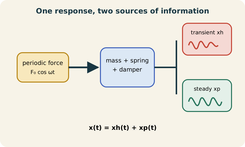
Linearity means responses can be added. If $x_h$ solves the homogeneous equation $mx''+cx'+kx=0$ and $x_p$ is one particular solution of the forced equation, then $x=x_h+x_p$ solves the complete equation. The subscripts mean homogeneous and particular. Each part answers a different modeling question. This decomposition is the mathematical foundation for transient-plus-steady language.

The transient remembers the initial state

The homogeneous response is governed by the characteristic equation $mr^2+cr+k=0$. Its roots determine whether the transient oscillates, decays without oscillating, or occupies a repeated-root boundary. In a stable damped system with $m>0$, $c>0$, and $k>0$, both root real parts are negative. The transient therefore fades as time increases. Initial displacement and velocity determine its constants.

For an underdamped system, the transient has the form $e^{-ct/(2m)}(C_1\cos\omega_dt+C_2\sin\omega_dt)$. The constants $C_1$ and $C_2$ encode the starting state. The damped natural frequency is $\omega_d=\sqrt{\frac{k}{m}-\left(\frac{c}{2m}\right)^2}$. The exponential envelope decays because damping transfers mechanical energy away. Its oscillation frequency is generally not the forcing frequency.

Calling this response transient does not mean it is negligible immediately. It can dominate during startup and can produce large short-term motion when combined with the particular solution. A measurement taken too early may not reflect steady behavior. Engineers often specify a settling time before interpreting frequency response. The transient becomes small only after enough damping time has passed.

The steady response follows the input frequency

For a sinusoidal input, seek a sinusoidal particular response at the same angular frequency. The system is linear and time-invariant, so sine and cosine inputs generate sine and cosine outputs at their frequency. Amplitude and phase can change, but the steady response does not invent a different frequency. Natural-frequency content belongs to the homogeneous portion. Damping causes that content to fade.

Write the particular response as $x_p=A\cos(\omega t-\phi)$. The amplitude $A$ is a nonnegative displacement magnitude in meters. The phase lag $\phi$ measures how far the response trails the force in radians. The response reaches corresponding points later when $\phi>0$. Amplitude and phase both depend on driving frequency.

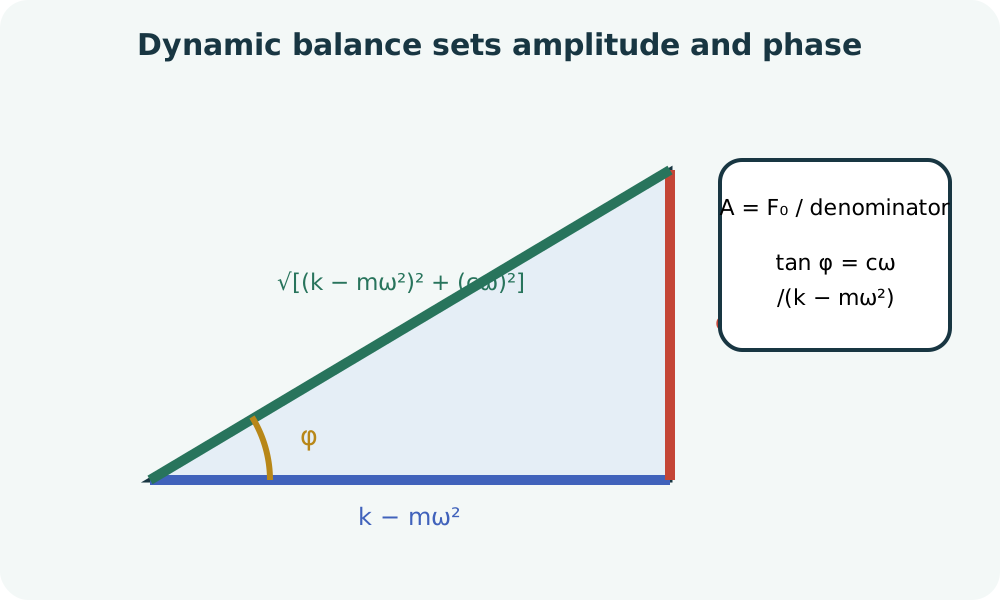
An equivalent form is $x_p=C\cos\omega t+D\sin\omega t$. Coefficient matching is often simpler in this form. The amplitude is $A=\sqrt{C^2+D^2}$. A correctly chosen angle satisfies $C=A\cos\phi$ and $D=A\sin\phi$. Quadrant information must be preserved when recovering phase.

Deriving amplitude by coefficient matching

Start with $x_p=C\cos\omega t+D\sin\omega t$. Then $x_p'=-C\omega\sin\omega t+D\omega\cos\omega t$. A second derivative gives $x_p''=-C\omega^2\cos\omega t-D\omega^2\sin\omega t$. Substitute all three expressions into the governing equation. Collect cosine and sine coefficients separately.

The cosine coefficient equation is $(k-m\omega^2)C+c\omega D=F_0$. The sine coefficient equation is $(k-m\omega^2)D-c\omega C=0$. These two linear equations determine $C$ and $D$. The combination $k-m\omega^2$ compares stiffness with inertia at the driving frequency. The term $c\omega$ measures the damping contribution at that frequency.

Solving and combining the coefficients gives $A(\omega)=\frac{F_0}{\sqrt{(k-m\omega^2)^2+(c\omega)^2}}$. The notation $A(\omega)$ emphasizes that amplitude is a function of driving frequency. The denominator has units of newtons per meter. Dividing force by that quantity leaves meters. The formula therefore returns displacement amplitude as required.

Deriving the phase relation

The phase relation follows from the coefficient ratio. A compact statement is $\tan\phi=\frac{c\omega}{k-m\omega^2}$. The numerator and denominator have the same units, so their ratio is dimensionless. A tangent value alone does not identify the correct quadrant. Both signs or a two-argument arctangent should be used.

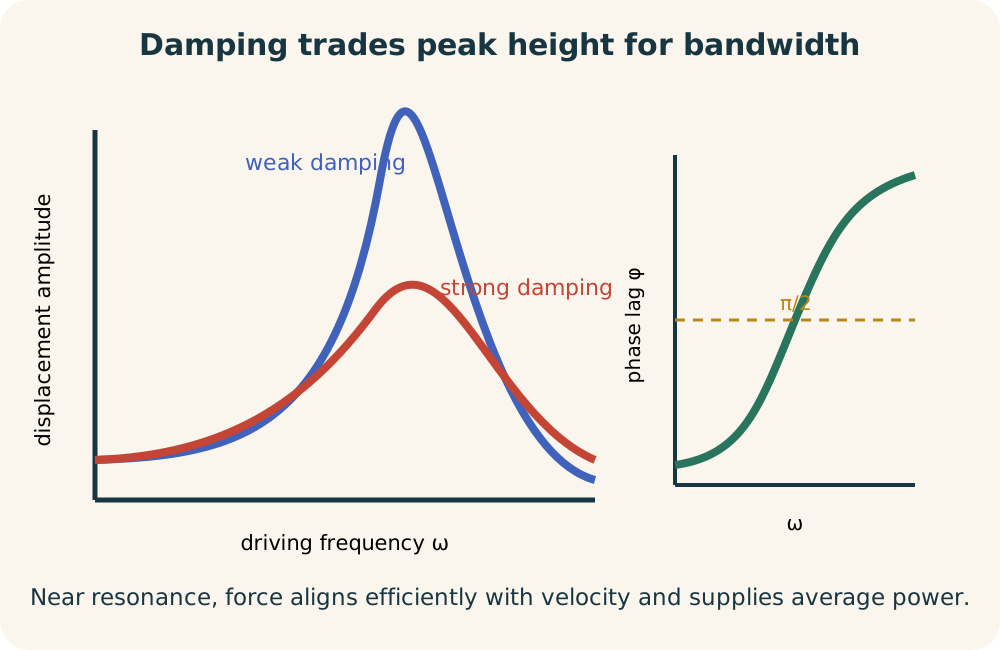
At very low frequency, $k-m\omega^2$ is positive and damping contribution is small. The phase lag approaches zero, so displacement is nearly in phase with force. Near the stiffness-inertia balance, the lag is near $\frac{\pi}{2}$. At very high frequency, the denominator is negative and the lag approaches $\pi$. The mass then moves nearly opposite the applied force.

Phase is not merely decorative information on a plot. Instantaneous power depends on force and velocity timing. Since velocity leads displacement by a quarter cycle for a sinusoid, the force-displacement phase controls average energy input. The strongest average transfer occurs when force aligns with velocity. Resonance is therefore deeply connected to phase.

Low-frequency behavior

When $\omega$ approaches zero, inertia $m\omega^2$ and damping $c\omega$ become small. The amplitude approaches $\frac{F_0}{k}$. This is the static extension produced by a slowly varying force. The system has time to remain near quasi-static equilibrium. Stiffness controls the response.

This limit provides a powerful check. A formula predicting zero displacement for a slowly applied nonzero force would contradict Hooke’s-law balance. Increasing stiffness lowers the low-frequency amplitude. Changing mass has little effect in the limit. These conclusions can be predicted without calculus.

The word slowly is relative to the system’s natural time scale. A frequency small for a stiff light oscillator may not be small for a soft massive one. Dimensionless frequency ratio $r=\frac{\omega}{\omega_0}$ makes this comparison explicit. Here $\omega_0=\sqrt{\frac{k}{m}}$ is the undamped natural angular frequency. A low-frequency regime means $r\ll1$.

High-frequency behavior

At very large $\omega$, the inertia term $m\omega^2$ dominates the amplitude denominator. The displacement amplitude approaches $\frac{F_0}{m\omega^2}$. It decreases with the square of frequency. The mass cannot follow rapidly reversing force with large displacement. Inertia controls the response.

The phase lag approaches $\pi$, or 180 degrees. When force points one way, displacement is nearly opposite because acceleration must follow the force while displacement relates through two time derivatives. Velocity and acceleration response can still be important even when displacement is small. A small position oscillation can therefore accompany a meaningful inertial load. Measurement choice affects which high-frequency behavior appears significant.

This limit also checks the formula. A larger mass makes high-frequency displacement smaller. Damping becomes less important than the $omega^2$ inertia term at sufficiently large frequency. Stiffness becomes comparatively negligible. The three mechanisms dominate in different frequency ranges.

Resonance and the amplitude peak

Between low and high frequency, $k-m\omega^2$ can approach zero. The stiffness and inertia contributions then nearly cancel in the amplitude denominator. Damping remains and prevents a zero denominator when $c>0$. The displacement response can become much larger than the static deflection. This frequency-sensitive amplification forms the resonance peak.

The undamped natural frequency is $\omega_0=\sqrt{\frac{k}{m}}$. With weak damping, the displacement peak lies near this value. For the viscously damped displacement response, the peak frequency is $\omega_r=\omega_0\sqrt{1-2\zeta^2}$ when $\zeta<\frac{1}{\sqrt{2}}$. The damping ratio is $\zeta=\frac{c}{2\sqrt{mk}}$. Stronger damping can remove a distinct displacement-amplitude peak.

This result corrects the oversimplification that resonance always occurs exactly at $\omega_0$. The exact peak depends on the measured response and damping. Velocity amplitude can peak at a different frequency, and acceleration has its own behavior. In weak damping the differences may be small. In careful work, resonance must be defined by the response quantity being maximized.

Undamped exact resonance

Set $c=0$ and drive at $\omega=\omega_0$. The steady-amplitude formula would divide by zero, so it is not valid as a finite periodic particular solution there. Direct solution produces a term proportional to $t\sin\omega_0t$. The amplitude envelope grows linearly with time. Energy accumulates because no damping removes it.

The growth is not exponential instability. It results from repeated in-phase energy addition at exact frequency match. Each cycle supplies another increment under the ideal constant-amplitude force. The response remains oscillatory while its envelope expands. Initial conditions alter the accompanying homogeneous motion but do not remove the resonant mechanism generically.

Real systems do not grow without limit. Material nonlinearities, changing damping, finite driver power, geometric stops, or failure eventually invalidate the ideal linear model. The mathematical divergence is a warning about omitted mechanisms. It identifies where the approximation must be revised. It should not be interpreted as a literal prediction of infinite displacement.

Energy transfer and phase

Instantaneous input power is $P(t)=F(t)x'(t)$. For steady sinusoidal response, the average over one cycle depends on the phase between force and velocity. If force is always perpendicular in phase-space timing to velocity, positive and negative work can cancel. When force tends to align with velocity, positive energy transfer accumulates. Damping dissipates the supplied energy.

In steady state, average mechanical energy stored in the oscillator repeats each cycle. Its net change over a full cycle is zero. Average input power therefore equals average power dissipated by the damper. For viscous damping, instantaneous dissipation is $c(x')^2$. This equality explains why a larger resonant response requires greater supplied power.

At resonance in a lightly damped system, the displacement lag is near $\frac{\pi}{2}$. Velocity is then nearly in phase with force. The driver does positive work efficiently. Away from resonance, timing is less favorable and more supplied energy is returned during other parts of the cycle. Resonant amplification is an energy-flow phenomenon expressed through phase.

Damping controls height and width

Increasing damping raises the $(c\omega)^2$ contribution in the denominator. The peak displacement becomes lower. The frequency range over which response is appreciable becomes broader. The system is less frequency-selective. This tradeoff is central to vibration control.

A lightly damped oscillator has a tall narrow peak. Small changes in driving frequency can cause large amplitude changes. A strongly damped oscillator has a lower, broader response. It does not amplify one narrow frequency as dramatically. The words sharp and broad refer to frequency width, not physical object shape.

Damping also shortens transient persistence. A weakly damped system can ring for many cycles after an input changes. A strongly damped system forgets its initial state more quickly, though excessive damping can make nonoscillatory return slow in time-domain problems. Frequency response and step response are related but not identical. Design goals must specify which behavior matters.

Bandwidth and quality factor

Bandwidth quantifies the width of a resonance region using a stated response criterion. A common power-based convention uses the two frequencies where average power is half its peak value. For lightly damped systems, the bandwidth $\Delta\omega$ is approximately related to damping. Narrow bandwidth means strong selectivity. Broad bandwidth means weak selectivity.

The quality factor $Q$ is often approximated by $Q\approx\frac{\omega_0}{\Delta\omega}$ for a lightly damped oscillator. It can also be related to damping ratio by $Q\approx\frac{1}{2\zeta}$. A large $Q$ means weak damping and a sharp response. A small $Q$ means stronger damping and a broader response. These approximations require the regime and convention to be stated.

Quality factor also has an energy interpretation. It compares energy stored with energy lost per cycle up to a conventional factor involving $2\pi$. A system that loses little energy each cycle can build a large resonant amplitude. A system that loses much energy cannot store as much under the same input. Frequency selectivity and energy retention describe the same underlying damping behavior.

Worked frequency-response example

Let $m=1.00\,\mathrm{kg}$, $k=100\,\frac{\mathrm{N}}{\mathrm{m}}$, $c=2.00\,\frac{\mathrm{N\,s}}{\mathrm{m}}$, and $F_0=5.00\,\mathrm{N}$. The natural angular frequency is $\omega_0=\sqrt{\frac{k}{m}}=10.0\,\frac{\mathrm{rad}}{\mathrm{s}}$. The damping ratio is $\zeta=\frac{2.00}{2\sqrt{(1.00)(100)}}=0.100$. The system is lightly damped. A distinct displacement peak is expected near the natural frequency.

At $\omega=10.0\,\frac{\mathrm{rad}}{\mathrm{s}}$, the stiffness-inertia term is $k-m\omega^2=0$. The amplitude is $A=\frac{5.00\,\mathrm{N}}{(2.00\,\frac{\mathrm{N\,s}}{\mathrm{m}})(10.0\,\mathrm{s^{-1}})}=0.250\,\mathrm{m}$. The static deflection is $\frac{F_0}{k}=0.0500\,\mathrm{m}$. Their ratio is dimensionless. The response at this frequency is five times the static deflection.

The phase lag at stiffness-inertia balance is $\frac{\pi}{2}$. The exact displacement-peak frequency is slightly below $10.0\,\frac{\mathrm{rad}}{\mathrm{s}}$ because damping is nonzero. Using $\omega_r=\omega_0\sqrt{1-2\zeta^2}$ gives approximately $9.90\,\frac{\mathrm{rad}}{\mathrm{s}}$. The shift is small because the damping ratio is small. It would become more noticeable with greater damping. This difference illustrates why “near natural frequency” is often more accurate than “exactly equal.”

Response measures are not interchangeable

Displacement amplitude is $A(\omega)$. Velocity amplitude is $\omega A(\omega)$ because differentiating a sinusoid multiplies amplitude by angular frequency. Acceleration amplitude is $\omega^2A(\omega)$. Multiplication by these frequency factors changes the locations and shapes of response peaks. A plot must label its response variable.

Structural clearance problems may prioritize displacement. Fatigue or damping devices may relate strongly to velocity. Inertial loads and human vibration exposure may prioritize acceleration. The same physical system can look safe by one measure and concerning by another. “The resonance frequency” is incomplete without context.

Electrical analogies show the same distinction. Charge, current, and voltage responses in a resistor-inductor-capacitor circuit correspond to different mechanical measures. A peak in current need not coincide with a peak in capacitor voltage under every condition. Mathematical transfer functions depend on selected input and output. Resonance is a property of a specified response relationship.

Applications and responsible design

Musical instruments use resonance to amplify selected frequencies. The instrument’s body and air cavities shape amplitude, phase, and radiation. Damping controls sustain and tone. Resonance is beneficial because the design directs it toward desired modes. The word resonance does not mean failure.

Structures and machines often require resonance control. Designers can shift natural frequencies by changing stiffness or mass. They can add damping to limit amplitude or isolate a system from troublesome operating frequencies. Tuned mass dampers add a secondary oscillator to redirect energy. Operating schedules can also avoid sustained driving near sensitive bands. Each strategy changes the governing dynamics rather than merely “avoiding vibration.”

Resonance can also reveal system properties. Sweeping an input frequency and measuring amplitude and phase can estimate natural frequencies and damping. Medical imaging, spectroscopy, sensors, and nondestructive testing use related frequency-sensitive responses. Interpretation requires calibrated models and appropriate response variables. The peak is data, not a complete explanation by itself.

Common mistakes and repairs

One mistake says the steady response oscillates at the natural frequency. In a linear damped system with sinusoidal forcing, the particular steady response follows the forcing frequency. Natural-frequency components appear in the transient. They decay when the system is stable and damped. Separate the two solution parts before interpreting a graph.

Another mistake says resonance always occurs exactly at $\sqrt{k/m}$. That value is the undamped natural frequency. The displacement peak shifts with damping, and other response measures can peak elsewhere. Define the measured quantity and damping regime. Use an appropriate peak condition rather than an unqualified slogan.

A third mistake attributes output energy to resonance itself. Resonance improves timing of energy transfer from a source. The driver still supplies energy, and damping or other loads receive it. An undamped ideal model accumulates energy because no loss mechanism exists. Always identify the energy source and system boundary.

Practice and retrieval

For $m=2.00\,\mathrm{kg}$, $k=72.0\,\frac{\mathrm{N}}{\mathrm{m}}$, and $c=6.00\,\frac{\mathrm{N\,s}}{\mathrm{m}}$, calculate $\omega_0$ and $\zeta$. Predict whether a distinct displacement peak exists using the stated criterion. Explain the roles of mass, stiffness, and damping. Compare the damping ratio with the peak threshold. Include units in every dimensional quantity.

For the same system with $F_0=12.0\,\mathrm{N}$, calculate steady displacement amplitude at $\omega=3.00\,\frac{\mathrm{rad}}{\mathrm{s}}$. Identify the stiffness-minus-inertia term and damping term separately. Determine phase quadrant. Compare the result with static deflection $F_0/k$. Interpret rather than merely reporting a number.

Finally, explain why force is nearly in phase with velocity near weakly damped resonance. Connect that timing with positive average power. Describe what damping does to the supplied energy. Explain why an undamped exact-resonance model grows without a finite steady amplitude. State one real mechanism that would eventually invalidate the linear model.

Solutions and reasoning

The natural angular frequency is $\omega_0=\sqrt{\frac{72.0\,\frac{\mathrm{N}}{\mathrm{m}}}{2.00\,\mathrm{kg}}}=6.00\,\frac{\mathrm{rad}}{\mathrm{s}}$. The damping ratio is $\zeta=\frac{6.00}{2\sqrt{(2.00)(72.0)}}=0.250$. Since this is below $\frac{1}{\sqrt{2}}$, a displacement peak exists. Mass supplies inertia, stiffness supplies restoration, and damping removes mechanical energy. Their relative scales determine the frequency response.

At $\omega=3.00\,\frac{\mathrm{rad}}{\mathrm{s}}$, $k-m\omega^2=72.0-18.0=54.0\,\frac{\mathrm{N}}{\mathrm{m}}$ and $c\omega=18.0\,\frac{\mathrm{N}}{\mathrm{m}}$. The amplitude is $A=\frac{12.0}{\sqrt{54.0^2+18.0^2}}=0.211\,\mathrm{m}$. Static deflection is $0.1667\,\mathrm{m}$. Both phase numerator and denominator are positive, so the lag lies in the first quadrant. Dynamic response is already amplified but remains below the resonance region.

Near weakly damped resonance, displacement lags force by about a quarter cycle, so velocity aligns with force. Their product is positive for much of the cycle, producing positive average input power. Damping transfers that energy out of the mechanical account. With no damping at exact resonance, coherent additions accumulate and the ideal amplitude envelope grows. Nonlinear stiffness, limited driver power, friction changes, geometric stops, or damage can end that prediction in a real system.

Connection forward

Forced oscillations connect naturally to transfer functions. A transfer function records amplitude and phase as functions of frequency. Poles encode characteristic roots, while the chosen numerator encodes the measured output. This language extends to circuits, controls, acoustics, and structures. The scalar oscillator provides a concrete foundation.

Multiple-degree-of-freedom systems contain several natural modes. A forcing pattern couples strongly to some modes and weakly to others. Frequency alone does not determine response because spatial mode shape matters. Damping can differ by mode. Resonance analysis then becomes a modal superposition problem.

Carry forward a disciplined statement. The transient remembers initial conditions and is governed by characteristic roots. The steady response follows the forcing frequency and has amplitude and phase set by dynamic balance. Resonance describes efficient frequency-dependent energy transfer in a specified input-output relationship. Damping limits, broadens, and phase-shifts that response.