Second-Order Oscillation Models

An oscillation model is more than an equation that produces a wavy graph. It is a compact account of inertia, restoring forces, energy loss, external inputs, and the information needed to predict motion. A second-order equation appears because acceleration is the second derivative of position and Newton’s second law connects acceleration to force. The model therefore preserves both where an object begins and how it is moving at that instant. This lesson develops that structure instead of treating formulas as disconnected facts.

Learning objectives

By the end of the lesson, you should be able to construct a second-order oscillator equation from a force diagram. You should be able to explain the physical meaning and units of every coefficient and variable. You should also distinguish displacement, velocity, acceleration, state, equilibrium, transient response, and steady response. Those distinctions are essential because different parts of a solution answer different physical questions. The goal is not merely to recognize the equation but to reason from a physical system to a defensible model.

You will classify free motion by comparing damping with inertia and stiffness. You will interpret the characteristic equation without treating its roots as unexplained algebraic machinery. You will use energy to explain why undamped motion persists and damped motion decays. You will then examine how an external force creates a frequency-dependent steady response. Each result will be checked against units, limiting cases, and qualitative expectations.

Keep one organizing question in mind throughout the lesson: what mechanism produces each mathematical term? The mass term records resistance to changes in motion, the damping term records velocity-dependent loss, and the stiffness term records displacement-dependent restoration. The forcing term records an influence imposed from outside the modeled system. Initial conditions specify the state from which those mechanisms begin acting. This mechanism-first approach makes unfamiliar oscillator equations easier to interpret and less tempting to memorize blindly.

From a force ledger to a differential equation

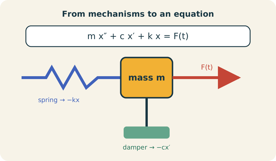
Consider a mass that moves horizontally while attached to a spring and a viscous damper. Let $x(t)$ denote displacement from equilibrium in meters, where $t$ is time in seconds. Its velocity is $x'(t)$ in meters per second, and its acceleration is $x''(t)$ in meters per second squared. A spring with stiffness $k$ exerts the restoring force $-kx$, whose negative sign points opposite the displacement. A damper with coefficient $c$ exerts the resistive force $-cx'$, whose negative sign points opposite the velocity.

Newton’s second law says that the sum of forces equals mass times acceleration. If an external force $F(t)$ acts in the positive direction, the force ledger is $F(t)-cx'-kx=mx''$. This ledger keeps the selected positive direction visible in every sign. The leftward internal forces appear negative before the terms are rearranged. That sign convention must remain unchanged throughout the derivation. Moving the internal-force terms to the left gives

$$m x''(t)+c x'(t)+k x(t)=F(t).$$

Here $m$ is mass in kilograms, $c$ is damping in newton-seconds per meter, and $k$ is stiffness in newtons per meter. Every term has units of newtons, so the equation is dimensionally consistent. The coefficient $m$ multiplies acceleration rather than velocity or position. The coefficient $c$ multiplies velocity because the assumed damper force depends on motion rate. The coefficient $k$ multiplies displacement because the assumed spring force depends on deformation.

The diagram below translates mechanisms into mathematical terms. The equation is not selected simply because it looks familiar. It is assembled from a signed force balance and constitutive rules for the spring and damper. The spring rule $F_s=-kx$ is Hooke’s law, while $F_d=-cx'$ is an ideal linear resistance rule. If either rule fails for a real device, the governing equation must change.

Why the equation is second order

The highest derivative is $x''$, so the equation is second order. That order has a physical meaning because knowing position alone does not determine what happens next. A mass at $x=0.050\,\mathrm{m}$ might be moving toward equilibrium, moving away from equilibrium, or momentarily at rest. Those possibilities share a position but have different velocities and therefore different futures. A unique prediction requires two independent initial conditions, usually $x(0)=x_0$ and $x'(0)=v_0$.

The pair $(x,v)$, where $v=x'$, is called the mechanical state. Position tells where the mass is, while velocity tells how its position is changing. Acceleration follows from the model as $x''=\frac{F(t)-cx'-kx}{m}$. The symbol $x_0$ denotes initial displacement in meters, and $v_0$ denotes initial velocity in meters per second. Once parameters, forcing, and these state values are known, the ideal model determines the future state.

This requirement provides a useful check on proposed solutions. A formula containing only one adjustable constant cannot generally satisfy two independent initial conditions. Two constants are expected in the general solution of a second-order linear equation. Those constants are not additional physical mechanisms because they encode the selected initial state. Thinking in terms of state explains why second-order motion requires two pieces of starting information.

Equilibrium and coordinate choice

An equilibrium is a state that can remain unchanged when external conditions are constant. At equilibrium, velocity and acceleration are zero, so a constant force $F_e$ gives $kx_e=F_e$. The symbol $x_e$ is equilibrium displacement measured from the original origin. If there is no constant applied force in the horizontal model, then $F_e=0$ and $x_e=0$. A sensible coordinate choice often places zero at equilibrium so the equations become easier to read.

A vertical spring illustrates why this shift matters. Gravity contributes the constant downward force $mg$, where $g$ is gravitational acceleration in meters per second squared. If downward is positive, the equation may be $my''+cy'+ky=mg$. The equilibrium position satisfies $ky_e=mg$, so $y_e=\frac{mg}{k}$. Defining $x=y-y_e$ removes the constant gravitational term and produces $mx''+cx'+kx=0$.

Gravity has not disappeared after this coordinate shift. It helped determine the equilibrium extension about which the mass oscillates. The shifted equation describes deviations from that already-stretched position. This is a general modeling move: locate equilibrium first and measure small motion relative to it. Doing so separates static balance from dynamic change and prevents a constant load from being mistaken for a driver.

The undamped natural oscillator

Set $c=0$ and $F(t)=0$ to isolate inertia and stiffness. The model becomes $mx''+kx=0$, or $x''+\frac{k}{m}x=0$ after division by mass. Define the natural angular frequency as $\omega_0=\sqrt{\frac{k}{m}}$. The symbol $\omega_0$ is measured in radians per second, although the radian is dimensionless in unit calculations. The corresponding frequency is $f_0=\frac{\omega_0}{2\pi}$ in hertz, and the period is $T_0=\frac{2\pi}{\omega_0}$ in seconds.

The free response is $x(t)=A\cos(\omega_0t)+B\sin(\omega_0t)$. The constants $A$ and $B$ have units of meters because sine and cosine are dimensionless. Applying $x(0)=x_0$ gives $A=x_0$, while applying $x'(0)=v_0$ gives $B=\frac{v_0}{\omega_0}$. The completed solution is $x(t)=x_0\cos(\omega_0t)+\frac{v_0}{\omega_0}\sin(\omega_0t)$. Both terms have units of meters, which is another valuable consistency check.

The word natural does not mean that every real oscillator moves forever at this frequency. It identifies the intrinsic frequency of the ideal undamped, unforced linear model. Increasing stiffness raises $\omega_0$ because a stronger restoring force reverses motion more quickly. Increasing mass lowers $\omega_0$ because greater inertia makes acceleration harder to produce. These trends can be predicted before arithmetic and help reveal inverted ratios.

Energy explains persistent oscillation

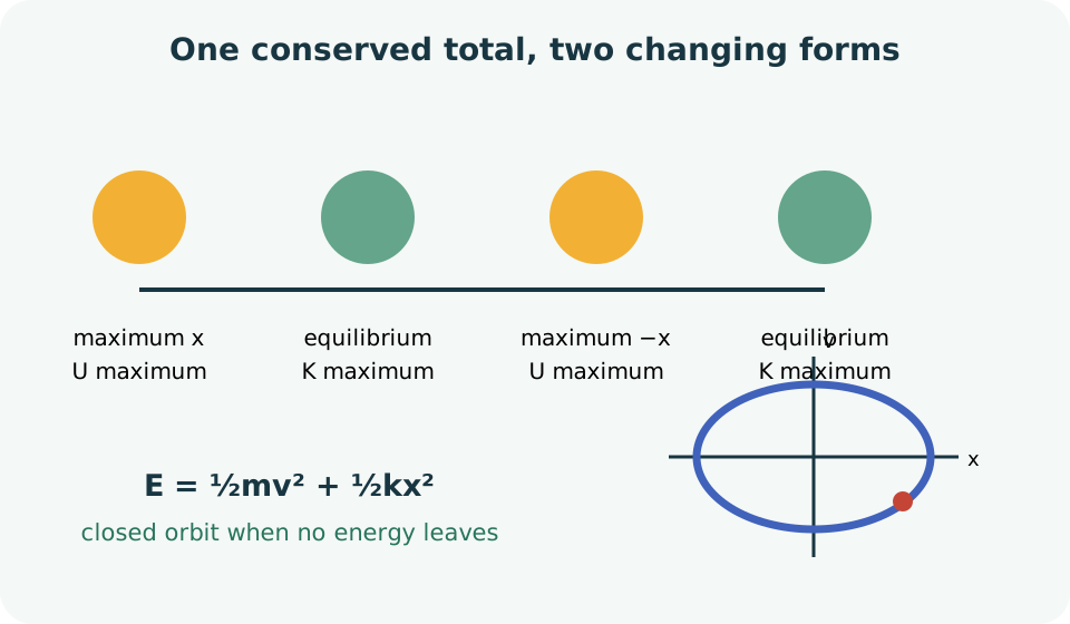
The undamped system continually trades kinetic energy for elastic potential energy. Its kinetic energy is $K=\frac{1}{2}m(x')^2$, where motion makes energy positive regardless of direction. Its spring potential energy is $U=\frac{1}{2}kx^2$, where displacement in either direction stores energy. The total is $E=\frac{1}{2}m(x')^2+\frac{1}{2}kx^2$. Both terms have units of joules, equivalent to newton-meters.

Differentiate energy to obtain $E'=mx'x''+kxx'$. Factoring velocity gives $E'=x'(mx''+kx)$. The undamped equation says that the expression in parentheses equals zero. Consequently $E'=0$, so total mechanical energy is constant. Oscillation persists because energy changes form without leaving the modeled mechanical account.

At maximum displacement, velocity is zero and all mechanical energy is spring potential energy. At equilibrium, displacement is zero and all mechanical energy is kinetic energy. Between those locations, both forms are present. The state traces a closed curve in the position-velocity plane. The energy view explains the motion causally and supplies a strong check on analytic or numerical solutions.

Damping and energy loss

Retain the damper but remove forcing, giving $mx''+cx'+kx=0$. Differentiate the same mechanical energy and substitute the equation. The result is $\frac{dE}{dt}=-c(x')^2$. For a passive damper, $c>0$, so the right side is never positive. The damper removes mechanical energy whenever the mass is moving.

Removed mechanical energy is usually converted into internal energy of the damper and surroundings. It is misleading to say that energy simply vanishes. The mechanical account decreases while a broader energy account remains conserved. Because the rate contains $(x')^2$, the loss does not depend on whether velocity points left or right. Faster motion creates a larger instantaneous transfer rate in this viscous model.

The equation clarifies useful limiting cases. If $c=0$, then $dE/dt=0$ and the undamped result returns. If velocity is momentarily zero, the damper transfers no energy at that instant even if the spring is stretched. Large damping does not automatically mean a faster return because excessive resistance can make motion sluggish. Distinguishing possible returns requires comparison of $c$ with both $m$ and $k$.

Characteristic roots and regimes

Try a free solution $x=e^{rt}$, where $r$ is a growth or decay rate. Substitution into $mx''+cx'+kx=0$ gives the characteristic equation $mr^2+cr+k=0$. Its roots are $r=\frac{-c\pm\sqrt{c^2-4mk}}{2m}$. The discriminant $c^2-4mk$ determines whether the roots are complex, repeated, or distinct real numbers. Those alternatives produce visibly different kinds of motion.

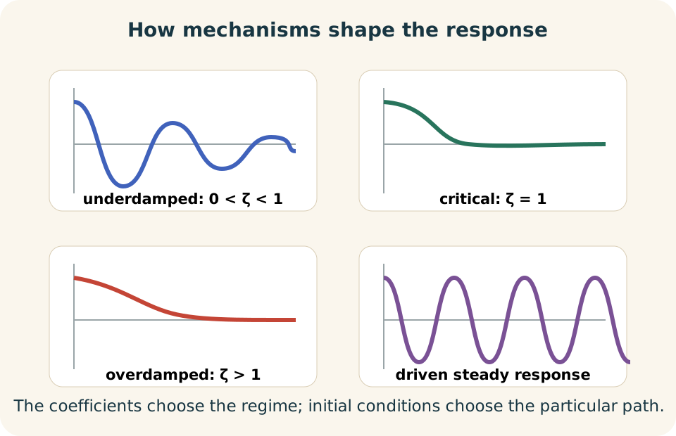
Define the dimensionless damping ratio as $\zeta=\frac{c}{2\sqrt{mk}}$. The Greek letter $\zeta$, pronounced zeta, compares actual damping with critical damping. When $0<\zeta<1$, complex roots create an underdamped response. When $\zeta=1$, a repeated root creates critical damping. When $\zeta>1$, two negative real roots create an overdamped response.

An underdamped system crosses equilibrium repeatedly while amplitude decays. A critically damped system returns without oscillating and lies at the boundary between oscillatory and nonoscillatory behavior. An overdamped system also avoids oscillation but usually returns more slowly because resistance dominates. Classification is therefore a comparison, not a judgment based on the numerical size of $c$ alone. A coefficient large for one mass-and-spring pair may be small for another.

Worked damping example

Suppose $m=2.00\,\mathrm{kg}$, $k=50.0\,\frac{\mathrm{N}}{\mathrm{m}}$, and $c=8.00\,\frac{\mathrm{N\,s}}{\mathrm{m}}$. The natural angular frequency is $\omega_0=\sqrt{\frac{k}{m}}=5.00\,\frac{\mathrm{rad}}{\mathrm{s}}$. Critical damping is $c_c=2\sqrt{mk}=20.0\,\frac{\mathrm{N\,s}}{\mathrm{m}}$. The damping ratio is $\zeta=\frac{c}{c_c}=0.400$. Because $0<0.400<1$, the motion is underdamped.

The underdamped envelope decays as $e^{-ct/(2m)}$. Here the exponential decay rate is $\frac{c}{2m}=2.00\,\mathrm{s}^{-1}$. After $t=1.00\,\mathrm{s}$, the amplitude envelope is multiplied by $e^{-2.00}=0.135$. This means displacement amplitude is about $13.5\%$ of the corresponding undamped envelope. It does not mean exactly $13.5\%$ of initial energy remains because energy scales with amplitude squared.

The damped angular frequency is $\omega_d=\omega_0\sqrt{1-\zeta^2}=4.58\,\frac{\mathrm{rad}}{\mathrm{s}}$. Its damped period is $T_d=\frac{2\pi}{\omega_d}=1.37\,\mathrm{s}$. Damping makes this frequency slightly lower than the undamped natural frequency. The calculation shows why units belong beside intermediate quantities rather than only at the final answer. Units reveal whether a number represents a rate, frequency, time, or dimensionless ratio.

External forcing and response parts

An input changes the equation to $mx''+cx'+kx=F(t)$. For sinusoidal forcing, write $F(t)=F_0\cos(\Omega t)$. The amplitude $F_0$ is measured in newtons, and driving angular frequency $\Omega$ is measured in radians per second. The complete solution has a transient part determined by the homogeneous equation and a particular part determined by the input. In stable damped systems, the transient decays while the forced steady response remains.

This decomposition is written $x=x_{\mathrm{transient}}+x_{\mathrm{steady}}$. The transient retains information about initial displacement and velocity. The steady response retains information about the continuing force, including amplitude and frequency. Calling one part transient does not make it unimportant because it may dominate after startup. Calling the other part steady does not mean the mass stops because steady response can be persistently oscillatory.

The sinusoidal steady displacement amplitude is $X(\Omega)=\frac{F_0}{\sqrt{(k-m\Omega^2)^2+(c\Omega)^2}}$. The symbol $X$ is a nonnegative amplitude in meters, not instantaneous signed displacement. The denominator has units of newtons per meter. Force divided by that denominator gives meters. This dimensional check confirms that the formula returns a displacement amplitude.

Resonance as a frequency relationship

At very low driving frequency, inertia and damping contribute little and $X\approx\frac{F_0}{k}$. This is the static spring extension produced by a slowly changing force. At very high frequency, inertia dominates and $X\approx\frac{F_0}{m\Omega^2}$, so displacement becomes small. Between those limits, cancellation between $k$ and $m\Omega^2$ can make the denominator comparatively small. That intermediate region produces the resonance peak.

Resonance is a frequency relationship, not merely a large applied force. Near resonance, the driver can add energy coherently over many cycles. Damping removes some energy each cycle and limits amplitude. Increasing damping generally lowers and broadens the displacement-response peak. With $c=0$ and driving exactly at $\omega_0$, the ideal model predicts growing amplitude rather than a finite steady response.

That unbounded prediction exposes a model boundary rather than predicting infinite real motion. A spring may become nonlinear, a structure may contact a stop, friction may change, or damage may occur. The source may also have finite power and fail to maintain its assumed force. Engineers use the linear resonance result as a warning and local approximation. They do not interpret mathematical divergence as permission to ignore constraints.

Auditing units, signs, and limits

Before trusting a model, audit the units of every term. Kilograms times meters per second squared makes newtons in $mx''$. Newton-seconds per meter times meters per second makes newtons in $cx'$. Newtons per meter times meters makes newtons in $kx$. The input $F(t)$ must also be in newtons for the sum to be meaningful.

Next test limiting cases because a sound expression should recover familiar behavior. Setting $c=0$ should produce undamped oscillation, while setting $F=0$ should produce free motion. Taking $k$ toward zero removes the restoring mechanism and an ordinary spring equilibrium. Increasing $m$ should reduce natural frequency rather than raise it. These checks often catch transcription errors faster than repeating algebra.

Finally compare signs and qualitative trends. Positive stiffness must create a force opposite displacement, and a passive positive damper must create a force opposite velocity. If a fitted model gives $c<0$, it represents energy input rather than passive loss and needs explanation. If a passive unforced solution grows, either its signs or assumptions deserve inspection. Model validation begins with this basic physical reasoning before sophisticated analysis.

Other systems with the same structure

A small-angle pendulum produces another second-order model. Its exact equation is $I\theta''+b\theta'+mg\ell\sin\theta=\tau(t)$, where $I$ is rotational inertia, $b$ is rotational damping, $\theta$ is angle, $\ell$ is length, and $\tau$ is torque. For small angles in radians, $\sin\theta\approx\theta$. That approximation turns the nonlinear equation into a linear oscillator. The stiffness-like coefficient is $mg\ell$ rather than a translational spring constant.

An electrical circuit provides another analogy. In a series resistor-inductor-capacitor circuit, charge can satisfy $Lq''+Rq'+\frac{1}{C}q=V(t)$. Inductance $L$ plays the mathematical role of inertia, resistance $R$ plays damping, and reciprocal capacitance $1/C$ plays stiffness. Voltage $V(t)$ acts like an external input. The analogy transfers reasoning even though the physical quantities and units differ.

These examples show why oscillator models recur across science and engineering. One storage mechanism analogous to inertia interacts with another analogous to stiffness, while dissipation or forcing may be added. The shared equation supports common tools and predictions. Nevertheless, an analogy never licenses careless substitution of units or interpretations. Identify what each symbol means in the actual system.

Linearization and model boundaries

The standard oscillator is linear because $x$, $x'$, and $x''$ appear only to the first power and are not multiplied together. Real restoring forces may contain $x^3$, and real drag may scale as $|x'|x'$. Such systems can show amplitude-dependent frequency, asymmetry, multiple equilibria, or complicated resonance. A linear model can remain useful near a stable equilibrium where departures are small. Its usefulness depends on scale and purpose, not on a claim of exact linearity.

Linearization replaces a smooth nonlinear force with a local tangent approximation. If restoring force is $R(x)$ near equilibrium $x_e$, then $R(x)\approx R(x_e)+R'(x_e)(x-x_e)$. The derivative $R'(x_e)$ supplies an effective local stiffness. Higher powers of displacement from equilibrium are neglected. The approximation must be checked against the displacement range actually reached.

A model also omits spatial complexity when it treats an object as a single mass. A long beam, string, or air column can possess many modes that vary across space. A one-coordinate oscillator may describe one dominant mode over a limited frequency range. At higher frequencies, additional modes may become important. Stating these boundaries makes the model more scientific, not less useful.

A repeatable workflow

Begin by defining the system boundary, coordinate, positive direction, and equilibrium. List every relevant force and determine its sign before inserting algebra. Apply Newton’s second law and arrange terms in a consistent form. Record the meaning and units of every parameter beside the model. Supply two initial conditions because the equation is second order.

Next simplify deliberately rather than automatically. Decide whether forcing is absent, damping is negligible, angles are small, or motion remains near equilibrium. Analyze the equation while keeping transient and steady contributions conceptually distinct. Check units at the equation level and for each derived quantity. Test limiting cases and compare predicted trends with physical intuition.

Finally compare the prediction with observations appropriate to the purpose. Disagreement might indicate incorrect parameters, poor initial conditions, an omitted force, nonlinearity, or measurement error. Do not repair disagreement by changing coefficients without explaining their physical meaning. A successful model connects mechanism, mathematics, measurement, and limitations. That is the transferable skill this lesson is designed to build.

Practice and retrieval

For $m=0.500\,\mathrm{kg}$ and $k=18.0\,\frac{\mathrm{N}}{\mathrm{m}}$, calculate $\omega_0$ and $T_0$ with units. Explain why doubling mass does not halve angular frequency. Identify the two initial conditions needed for free motion. State which part of a damped forced response preserves those initial conditions. These tasks combine computation with interpretation instead of rewarding recall alone.

Suppose $c=6.00\,\frac{\mathrm{N\,s}}{\mathrm{m}}$ for that system. Compute $c_c=2\sqrt{mk}$ and $\zeta=\frac{c}{c_c}$. Use $\zeta$ to classify the response. Predict whether the mass crosses equilibrium after release from rest. Explain how the energy equation supports your prediction about eventual motion.

Choose a pendulum, vehicle suspension, loudspeaker cone, or electrical circuit for a transfer task. Identify inertia, damping, stiffness, forcing, response, and initial state. State one approximation required to obtain a linear model. Describe an observation that would signal failure of that approximation. This exercise tests whether you can carry the structure into a new setting.

Solutions and reasoning

For the first system, $\omega_0=\sqrt{\frac{18.0\,\frac{\mathrm{N}}{\mathrm{m}}}{0.500\,\mathrm{kg}}}=6.00\,\frac{\mathrm{rad}}{\mathrm{s}}$ and $T_0=\frac{2\pi}{\omega_0}=1.05\,\mathrm{s}$. Doubling mass multiplies frequency by $\frac{1}{\sqrt{2}}$ because mass lies under a square root. The initial conditions are displacement and velocity at the same time. The transient preserves that information. In a stable damped system, it fades as the transient decays.

Here $c_c=2\sqrt{(0.500\,\mathrm{kg})(18.0\,\frac{\mathrm{N}}{\mathrm{m}})}=6.00\,\frac{\mathrm{N\,s}}{\mathrm{m}}$. Therefore $\zeta=1.00$, indicating critical damping. The ideal critically damped response returns without crossing equilibrium after release from rest. Mechanical energy decreases because $\frac{dE}{dt}=-c(x')^2\leq0$. Eventually displacement and velocity approach zero in the unforced model.

A correct transfer answer names mechanisms rather than merely relabeling symbols. For a vehicle, mass supplies inertia, the shock absorber supplies damping, the spring supplies stiffness, and road motion supplies input. Body displacement and velocity form the state, while linearity assumes modest travel. Bottoming out or amplitude-dependent response would expose model failure. Other systems can be analyzed with the same logic and their own units.

Connection forward

This lesson treated one dominant coordinate, but many systems contain several interacting coordinates. Coupling produces multiple natural frequencies and mode shapes that lead toward standing waves. Periodic forcing selects among those modes according to frequency and spatial pattern. The same distinctions among inertia, restoration, damping, input, transient, and steady response still organize the analysis. Mastering one coordinate prepares you to reason about richer vibrating systems.

The characteristic equation connects directly to general second-order differential equations. Its roots determine whether the homogeneous response oscillates, decays, or grows. Repeated roots require a modified solution, while complex roots encode decay and rotation in state space. Those algebraic patterns are not detached from physics because they summarize competing mechanisms. Studying them in mathematical and physical language strengthens both views.

Most importantly, carry forward the habit of explaining every term. A formula becomes meaningful when its variables, units, signs, assumptions, and limits are explicit. A graph becomes meaningful when its axes and measured response are identified. A numerical answer becomes meaningful when it is checked against scale and mechanism. Oscillator models are valuable because they teach disciplined translation between physical reasoning and mathematics.