Standing Waves and Resonance

A wave can travel along a string, reflect, and overlap its returning copy. At particular frequencies, the superposition creates a stable spatial pattern of nodes and antinodes. This pattern is a standing wave. Energy continues moving and oscillators continue moving even though the pattern does not translate. Boundary conditions decide which patterns fit.

Resonance occurs when periodic driving couples efficiently to a natural mode. The response can become large because the driver adds energy with a favorable phase over many cycles. Damping removes energy and limits amplitude. A resonant frequency is therefore not merely “the frequency that destroys things.” It is a natural-response feature whose consequence depends on drive strength, duration, damping, and structure.

This lesson begins by adding opposite-traveling sinusoidal waves. It then derives string, open-pipe, and closed-pipe mode conditions. Displacement and pressure descriptions will be kept separate in sound. Harmonics, overtones, resonance curves, beats, and quality factor will connect equations to observation. Every mode formula will be tied to a drawn boundary condition.

Learning objectives and an opening prediction

After this lesson, you should identify nodes and antinodes in a standing wave. You should derive allowed wavelengths and frequencies for strings and air columns. You should distinguish harmonic number from overtone number. You should explain resonance as driven energy transfer with damping. You should also interpret resonance curves, beats, and experimental uncertainty.

Imagine a string fixed at both ends. Predict whether it can support a mode with a displacement antinode at an endpoint. The fixed support requires zero transverse displacement, so every allowed pattern must have a node there. Only wavelengths fitting an integer number of half-wavelengths into the length satisfy both ends. Boundary conditions filter the possibilities.

Now imagine an air column closed at one end and open at the other. The closed end is a displacement node, while the open end is approximately a displacement antinode. The shortest fitting pattern occupies one quarter of a wavelength. Only odd harmonics appear in the ideal uniform closed-pipe model. A different boundary produces a different spectrum.

Traveling waves superpose into a standing pattern

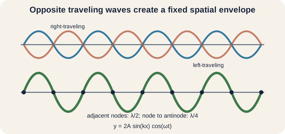
Consider equal waves traveling in opposite directions: $y_1=A\sin(kx-\omega t)$ and $y_2=A\sin(kx+\omega t)$. The symbol $A$ is amplitude, $k=\frac{2\pi}{\lambda}$ is wave number, and $\omega=2\pi f$ is angular frequency. Position is $x$ and time is $t$. The opposite signs before $\omega t$ encode opposite propagation directions. Their speeds have equal magnitude and opposite direction.

Add them using $\sin(\alpha-\beta)+\sin(\alpha+\beta)=2\sin\alpha\cos\beta$. The total is $y(x,t)=2A\sin(kx)\cos(\omega t)$. The spatial factor and time factor are separated. Every point oscillates with the same frequency but a position-dependent amplitude $2A|\sin(kx)|$. The envelope remains fixed in space.

At positions where $\sin(kx)=0$, displacement is always zero. These are nodes. Where $|\sin(kx)|=1$, oscillation amplitude is maximum and the points are antinodes. Adjacent nodes are separated by $\frac{\lambda}{2}$. A node-to-nearest-antinode distance is $\frac{\lambda}{4}$.

Standing does not mean motionless

The shape called a standing wave changes through time. At one instant, the string reaches one extreme profile. One quarter-period later, every point passes through equilibrium. Another quarter-period later, the profile is inverted. Nodes remain fixed while other points oscillate.

Points between adjacent nodes move in phase. Points in neighboring loops move in opposite phase because the spatial sine changes sign. The string does not transport a crest continuously from one end to the other in the standing pattern. Local kinetic and elastic energy exchange. Traveling components still carry energy in opposite directions.

An ideal pure standing wave has zero net time-averaged energy flow because equal traveling contributions oppose. Real driven systems receive energy from a source and lose energy through damping. Their pattern can be nearly standing while a small net energy flow supplies losses. Ideal language should not erase the energy pathway. Resonance requires ongoing transfer.

Reflection and boundary conditions

A pulse reflecting from a fixed string end inverts because the endpoint cannot move. The reflected displacement has opposite sign. At a free end, reflection does not invert in the same way because the transverse force condition differs. Repeated reflections combine with incident waves. Allowed modes are those that reproduce boundary requirements.

A fixed string endpoint imposes $y=0$, a displacement node. A freely moving ideal end imposes a zero-slope force condition and commonly acts as a displacement antinode. Air columns require pressure and air-displacement conditions. A rigid closed end prevents longitudinal air displacement. An open end remains near atmospheric pressure and therefore has a pressure node.

Boundary conditions are not decorative end labels. They determine mathematical solutions. Changing one end from fixed to free changes allowed wavelengths. Adding mass or compliance at an end creates an intermediate condition. Real instruments approximate ideal boundaries with corrections.

Strings fixed at both ends

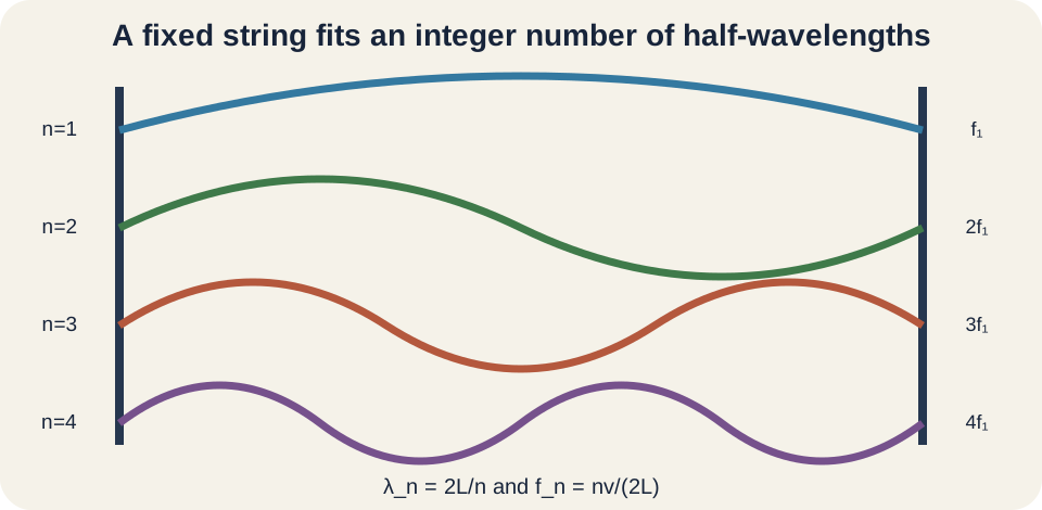
For a string of length $L$ fixed at both ends, each endpoint must be a displacement node. The length must contain an integer number of half-wavelengths: $L=n\frac{\lambda_n}{2}$. The positive integer $n=1,2,3,\ldots$ labels the harmonic. Solving gives $\lambda_n=\frac{2L}{n}$. Larger $n$ means shorter wavelength.

Using wave speed $v=\lambda f$, the allowed frequencies are $f_n=\frac{v}{\lambda_n}=\frac{nv}{2L}$. The fundamental is $f_1=\frac{v}{2L}$. Frequencies are integer multiples $f_n=nf_1$. The harmonic number $n$ is dimensionless. An ideal uniform fixed string therefore supports all positive-integer harmonics.

The $n$th mode contains $n$ half-wavelength loops, $n-1$ interior nodes, and $n$ antinodes. Endpoints add two more nodes. Counting loops is often the easiest way to identify $n$. Counting all nodes and calling that number the harmonic produces an error. A diagram should show which count is used.

String wave speed depends on tension and density

For an ideal flexible string, transverse wave speed is $v=\sqrt{\frac{T}{\mu}}$. Here $T$ is tension in newtons and $\mu$ is linear mass density in $\mathrm{\frac{kg}{m}}$. The symbol $T$ can also denote period elsewhere, so context and units matter. Greater tension increases speed. Greater mass per length decreases it.

Substitute into the harmonic formula: $f_n=\frac{n}{2L}\sqrt{\frac{T}{\mu}}$. Shorter strings, higher tension, and smaller linear density produce higher frequencies. Doubling tension raises frequency by $\sqrt{2}$, not by two. Quadrupling tension doubles frequency. Scaling checks make the square root meaningful.

Stringed instruments change effective length by pressing against a fingerboard or fret. Tuning pegs change tension. Different string thicknesses and materials change $\mu$. Real stiffness produces inharmonicity, especially in thick or short strings. The ideal model provides the first approximation to pitch.

Worked string example

A string of length $L=0.800\,\mathrm m$ supports waves at $v=240\,\mathrm{\frac{m}{s}}$. Its fundamental frequency is $f_1=\frac{240\,\mathrm{\frac{m}{s}}}{2(0.800\,\mathrm m)}=150\,\mathrm{Hz}$. Meters cancel, leaving inverse seconds or hertz. The second harmonic is $300\,\mathrm{Hz}$. The third is $450\,\mathrm{Hz}$.

The third-harmonic wavelength is $\lambda_3=\frac{2(0.800\,\mathrm m)}{3}=0.533\,\mathrm m$. The length contains three half-wavelengths. It has three antinodes and two interior nodes. Including fixed endpoints, it has four nodes total. Its frequency also follows $\frac{v}{\lambda_3}=450\,\mathrm{Hz}$.

If tension increases while length and $\mu$ remain fixed, every harmonic frequency scales by the same square-root factor. Harmonic ratios remain integer under the ideal model. The timbre can still change because driving and damping excite modes with different amplitudes. Frequency set and amplitude spectrum are different properties. A mode can be allowed but weakly excited.

Open pipes and displacement antinodes

An ideal pipe open at both ends has air-displacement antinodes near both openings. It also has pressure nodes there because pressure fluctuation remains near atmospheric. The fundamental fits one half-wavelength into the pipe: $L=\frac{\lambda_1}{2}$. Therefore $\lambda_n=\frac{2L}{n}$ and $f_n=\frac{nv}{2L}$. The ideal spectrum includes all integer harmonics.

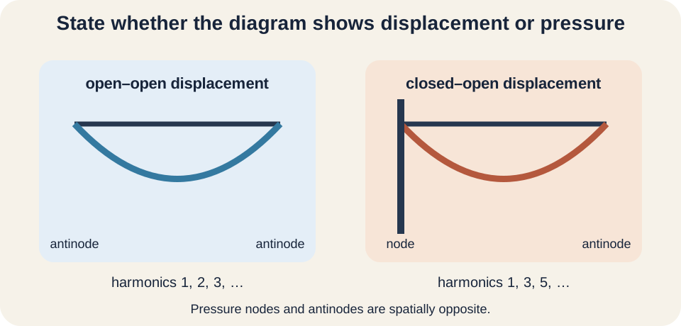
Air displacement and pressure are out of phase spatially by one quarter wavelength. A displacement antinode corresponds to a pressure node. A displacement node corresponds to a pressure antinode. Diagrams must declare which quantity is shown. Calling an open end simply “an antinode” without that declaration is ambiguous.

Real open ends radiate sound into surrounding air, so the displacement antinode lies slightly beyond the physical opening. An end correction makes effective acoustic length longer than geometric length. The correction depends on radius and end geometry. Introductory formulas often neglect it. Precision experiments should include or infer it.

Closed-open pipes select odd harmonics

An ideal pipe closed at one end and open at the other has a displacement node at the closed end and a displacement antinode at the open end. The fundamental contains one quarter wavelength: $L=\frac{\lambda_1}{4}$. Thus $\lambda_1=4L$ and $f_1=\frac{v}{4L}$. The next fitting pattern adds a half-wavelength. It contains three quarters of a wavelength.

Allowed lengths are $L=(2q-1)\frac{\lambda_q}{4}$ for $q=1,2,3,\ldots$. Frequencies are $f_q=(2q-1)\frac{v}{4L}$. Expressed as harmonics, the allowed multipliers are $1,3,5,\ldots$. Even harmonics are absent in the ideal uniform model. The second allowed mode is the third harmonic.

This naming causes common confusion. The first overtone is the next frequency above the fundamental. In a closed pipe, it is the third harmonic, not the second harmonic. The second overtone is the fifth harmonic. Overtone counts observed modes above the fundamental, while harmonic counts multiples of the fundamental. Always specify which label is being used.

Worked air-column example

An ideal closed-open pipe has length $0.850\,\mathrm m$ and sound speed $343\,\mathrm{\frac{m}{s}}$. Fundamental frequency is $f_1=\frac{343}{4(0.850)}=101\,\mathrm{Hz}$ to three significant figures. The first overtone is the third harmonic, $f_3=303\,\mathrm{Hz}$. The second overtone is the fifth harmonic, $505\,\mathrm{Hz}$. Even harmonics are excluded by the mixed boundary conditions.

An ideal open-open pipe of the same length has fundamental $f_1=\frac{343}{2(0.850)}=202\,\mathrm{Hz}$. Its first overtone is the second harmonic, $404\,\mathrm{Hz}$. Changing one boundary doubles the ideal fundamental in this comparison. The formulas share sound speed and length but differ in fitted fraction. Drawing the fundamental prevents denominator confusion.

Measured values may differ because of end correction, temperature-dependent sound speed, pipe diameter, and nonuniformity. Sound speed in air rises with temperature under ordinary conditions. A systematic frequency offset can reveal an incorrect effective length. Data should be compared with uncertainty. Model discrepancy can be physically informative.

Natural modes and resonance

A natural mode is a pattern in which a system can oscillate freely after a suitable disturbance. Each mode has a natural frequency determined by inertia, restoring behavior, geometry, and boundary conditions. A real initial disturbance can excite several modes at once. The resulting motion is their superposition. Fourier analysis separates the contributions.

Periodic driving applies force repeatedly. When drive frequency lies near a natural frequency, the driver can add energy coherently over many cycles. Response amplitude becomes relatively large. This is resonance. The precise peak depends on damping and on which quantity is measured.

Driving at a natural frequency does not guarantee a large response if the force pattern couples poorly to that mode. Pushing at a string node for a particular mode supplies little displacement work there. Symmetry can suppress coupling. Drive location and shape matter along with frequency. Resonance is a property of the driven system interaction.

Phase explains energy transfer

Instantaneous mechanical power from a drive is $P=\mathbf F\boldsymbol\cdot\mathbf v$. Positive average power requires a favorable relationship between driving force and velocity. Near resonance, system phase adjusts so the driver can supply energy effectively. Far from resonance, energy added during part of a cycle may be returned during another. Phase is therefore central to resonant response.

For a lightly damped oscillator, displacement lags the driving force by a phase that changes across resonance. At low frequency, displacement is nearly in phase with force. Near resonance, the lag is approximately one quarter cycle in the elementary model. At high frequency, it approaches half a cycle. Velocity phase differs from displacement phase by a quarter cycle.

The phrase “matching frequency adds energy each push” is useful but incomplete. Timing relative to velocity determines work. A push in the direction of motion adds energy; a push against it removes energy. Resonant phase locking maintains net positive transfer that balances damping in steady state. The amplitude stops growing when average input power equals average dissipated power.

Damping controls amplitude and width

Damping transfers organized oscillation energy into thermal, acoustic, or other accounts. Greater damping generally lowers the resonant peak and broadens the frequency response. Weak damping produces a tall narrow peak. The system remembers oscillation for many cycles. Strong damping produces a smaller, broader response.

Quality factor $Q$ can characterize a lightly damped resonance. One definition is $Q=\frac{f_0}{\Delta f}$, where $f_0$ is resonant frequency and $\Delta f$ is the full width between half-power points. The symbol $Q$ here is not volume flow rate or heat. It is dimensionless. Large $Q$ means narrow resonance and slow energy loss.

Another interpretation is proportional to energy stored divided by energy lost per cycle. A high-$Q$ tuning fork rings for a long time. A shock absorber is designed for substantial damping and low sustained oscillation. Desired damping depends on purpose. Musical sustain and structural stability seek different responses.

Resonance curves are evidence

Plot steady-state amplitude vertically against drive frequency horizontally. The curve rises toward a peak and falls away. The peak location estimates a resonant frequency under specified damping. The width quantifies selectivity. Axes need units and a named amplitude measure.

Amplitude is not identical to power. Half-power points correspond to power response dropping to one half of peak in standard lightly damped contexts. If measured amplitude squared is proportional to power, half power occurs at amplitude $\frac{1}{\sqrt{2}}$ of peak. Calling half-amplitude points the bandwidth would be incorrect. Measurement definition must match the formula.

Sweep rate can distort a resonance curve if the system has insufficient time to reach steady state. Nonlinear systems can show amplitude-dependent resonance, asymmetry, or hysteresis. Sensor loading can change damping. Repeated upward and downward sweeps test history dependence. An ideal Lorentzian-like curve is a model, not guaranteed data.

Beats reveal nearby frequencies

Add two sinusoidal waves with close frequencies $f_1$ and $f_2$. Trigonometric identities show a rapid oscillation multiplied by a slowly changing envelope. The beat frequency is $f_{\mathrm{beat}}=|f_1-f_2|$. Listeners perceive loudness rising and falling at this rate when the frequencies are close enough. The average carrier frequency is approximately $\frac{f_1+f_2}{2}$.

If tuning forks at $256\,\mathrm{Hz}$ and $260\,\mathrm{Hz}$ sound together, beat frequency is $4\,\mathrm{Hz}$. Loudness cycles four times each second. Adjusting one fork until beats slow to zero can tune frequencies to equality. The method measures difference more sensitively than absolute pitch. Phase drift creates the envelope.

Beats are not a new third physical source oscillating at $4\,\mathrm{Hz}$. They are amplitude modulation produced by superposition. A detector with nonlinear intensity response can reveal the envelope strongly. If frequencies are too far apart, the ear may hear separate tones rather than slow beats. Perception adds another layer.

Resonance in structures and safety

Buildings, bridges, vehicle suspensions, and machine parts have many natural modes. Wind, traffic, rotating machinery, or earthquakes can drive them. Engineers estimate modal frequencies, shapes, damping, and forcing spectra. Avoiding exact frequency coincidence is only one strategy. Increasing damping, changing stiffness, altering mass, or reducing forcing can also control response.

Resonance does not automatically cause failure. Stress amplitude must exceed material and fatigue limits for sufficient duration. Nonlinear behavior can shift frequencies, and damping limits response. Multiple modes may interact. Safety analysis requires validated structural models and measured loads.

The famous instruction that soldiers break step on a bridge reflects concern about coherent periodic forcing, but real bridge behavior is more complex than a single oscillator. Aeroelastic effects can involve feedback between motion and airflow. Tuned mass dampers add a secondary oscillator to reduce building response. Engineering designs use resonance deliberately as well as defensively. Context determines whether it is useful or hazardous.

Measuring modes in an experiment

A string experiment can vary drive frequency and record amplitude at a selected location. Sprinkle lightweight markers or use video to locate nodes. Measure string length and tension, and calculate linear density from mass per known length. Compare measured $f_n$ with $\frac{n}{2L}\sqrt{\frac{T}{\mu}}$. Plot frequency against harmonic number.

An ideal fixed string gives a straight line through the origin with slope $\frac{v}{2L}$. A nonzero intercept or curved residuals suggest boundary, stiffness, or calibration effects. Harmonic-number misidentification can create systematic errors. Use mode shape as well as frequency to label each point. Repeated trials estimate uncertainty.

For air columns, resonance can be detected by microphone amplitude while changing frequency or effective length. End correction shifts the relationship. Ambient temperature changes sound speed. Background reflections can create extra peaks. Report geometry and environmental conditions.

Common misconceptions and repairs

One misconception says standing-wave nodes contain no energy. Displacement is always zero there, but local tension forces and energy distribution require a more careful field description. In a string, different energy forms vary through the cycle. The total standing pattern is not empty at nodes. “No displacement” is the correct elementary statement.

Another misconception labels every next mode as the next harmonic. Open-open pipes and fixed strings support consecutive integer harmonics. Ideal closed-open pipes support odd harmonics only. Their first overtone is the third harmonic. Draw the boundary pattern before naming it.

A third misconception says resonance creates energy. The driver supplies energy, while resonance makes transfer efficient. Damping removes it. Steady resonant amplitude reflects an input-loss balance. Conservation remains intact.

Practice with guided feedback

First, find the first three frequencies of a $1.20\,\mathrm m$ fixed string with wave speed $180\,\mathrm{\frac{m}{s}}$. Second, find the first three allowed frequencies for a closed pipe of the same length with sound speed $343\,\mathrm{\frac{m}{s}}$. Third, identify displacement nodes at open and closed air-column ends. Fourth, explain how increased damping changes a resonance curve. Draw each fundamental boundary pattern before calculating.

The string fundamental is $\frac{180}{2(1.20)}=75.0\,\mathrm{Hz}$, followed by $150\,\mathrm{Hz}$ and $225\,\mathrm{Hz}$. The closed-pipe fundamental is $\frac{343}{4(1.20)}=71.5\,\mathrm{Hz}$, followed by odd harmonics $214\,\mathrm{Hz}$ and $357\,\mathrm{Hz}$. The closed end is a displacement node and open end a displacement antinode. Increased damping lowers and broadens the resonant peak. Every answer follows from a boundary drawing.

For a node-spacing check, adjacent nodes must be $\frac{\lambda}{2}$ apart. For a frequency check, verify $v=\lambda f$. For a naming check, distinguish harmonic from overtone. For an energy check, identify drive input and damping output. These checks join geometry, algebra, and physics.

Retrieval and connection forward

Without looking back, add opposite traveling waves to obtain a standing-wave form. Define nodes, antinodes, and their spacings. Derive modes for a fixed string, open pipe, and closed pipe. Explain why odd harmonics arise for mixed boundaries. Finish by connecting resonance amplitude, phase, damping, and quality factor.

Diffraction and interference use the same superposition principle in space. Fourier analysis decomposes complicated motion into normal modes. Quantum mechanics replaces classical mode energy with quantized oscillator states. Acoustics and musical instruments build timbre from harmonic spectra. Structural engineering treats many coupled modes and damping mechanisms.

Keep one organizing statement: standing waves are superpositions constrained by boundaries, so only fitting spatial modes and frequencies persist. Nodes and antinodes describe the chosen field, whether displacement or pressure. Resonance is efficient driven energy transfer near a natural mode. Damping limits amplitude and sets bandwidth. Geometry, phase, and energy accounting must all agree.