Damping Determines How Oscillations Fade

An ideal mass and spring can oscillate forever. Real systems lose organized mechanical energy through friction, drag, electrical resistance, internal material deformation, or deliberate damping devices. Their motion fades toward equilibrium. The manner of fading depends on the balance among inertia, damping, and restoring stiffness. A differential equation makes that balance quantitative.

The same mathematical model describes vehicle suspension motion, door closers, seismometers, instrument needles, and structural vibration. Some designs should settle rapidly without overshoot. Others should preserve oscillations long enough to measure frequency. The correct damping level depends on purpose. More damping is not automatically better.

This article derives all three free-response regimes from the characteristic roots. It explains damping ratio, natural frequency, decay envelope, damped frequency, initial conditions, energy loss, logarithmic decrement, and design tradeoffs. Every coefficient receives units and physical meaning. Three diagrams compare motion, roots, and energy. The goal is to read behavior directly from the model.

Build the mass–spring–damper equation

Let displacement $x(t)$ measure position from static equilibrium. A linear spring exerts restoring force $-kx$. A viscous damper exerts force $-cx'$. The prime means differentiation with respect to time. Both force signs oppose their associated displacement or velocity.

Newton’s second law gives $mx''=-cx'-kx$. Move every term to one side to obtain $mx''+cx'+kx=0$. Mass $m$ multiplies acceleration. Damping coefficient $c$ multiplies velocity. Spring stiffness $k$ multiplies displacement.

The right side is zero because no external driving force is included. This is free damped motion. Gravity may already be absorbed into the equilibrium reference for a vertical spring. Initial displacement and velocity start the motion. The coefficients determine the system response family.

Units make each term a force

Mass has unit kilograms, and acceleration has unit $\mathrm{\frac{m}{s^2}}$. Therefore $mx''$ has unit $\mathrm{\frac{kg\,m}{s^2}}=\mathrm N$. Stiffness has unit $\mathrm{\frac{N}{m}}$, so $kx$ also has newtons. Every term in one physical equation must share units. This check catches many transcription and modeling errors before calculation begins.

Velocity has unit $\mathrm{\frac{m}{s}}$. To make $cx'$ a force, damping coefficient has unit $\mathrm{\frac{N\,s}{m}}$. This is equivalent to $\mathrm{\frac{kg}{s}}$. A bare numerical value for $c$ is incomplete. Units distinguish physically different parameter scales.

Time has unit seconds in the common mechanical model. Characteristic roots therefore have unit $\mathrm{\frac{1}{s}}$. Their real parts are decay rates. Their imaginary parts are angular frequencies in $\mathrm{\frac{rad}{s}}$, where radians are dimensionless in SI. Dimensional checks constrain every derived formula.

Equilibrium and model assumptions

The equation’s equilibrium is $x=0$. Setting displacement, velocity, and acceleration to zero satisfies it. This equilibrium is stable when $m>0$, $c>0$, and $k>0$. Small disturbances decay. The state includes both position and velocity.

The model assumes linear spring force and viscous damping proportional to velocity. Coulomb friction, quadratic drag, hysteresis, and nonlinear stiffness require different terms. Parameters are treated as constant. The displacement is measured where the linear approximation is valid. Those assumptions define the domain in which conclusions from the equation deserve trust.

A useful model need not include every microscopic loss mechanism. Coefficient $c$ can represent an effective damping level over a range. Experimental data must test whether exponential decay is adequate. Residual patterns reveal systematic model failure. Mathematical precision does not guarantee physical completeness.

Characteristic roots organize the response

Try a solution $x=e^{rt}$. Its derivatives are $x'=re^{rt}$ and $x''=r^2e^{rt}$. Substitution gives $(mr^2+cr+k)e^{rt}=0$. Exponential $e^{rt}$ is never zero. Therefore roots satisfy $mr^2+cr+k=0$.

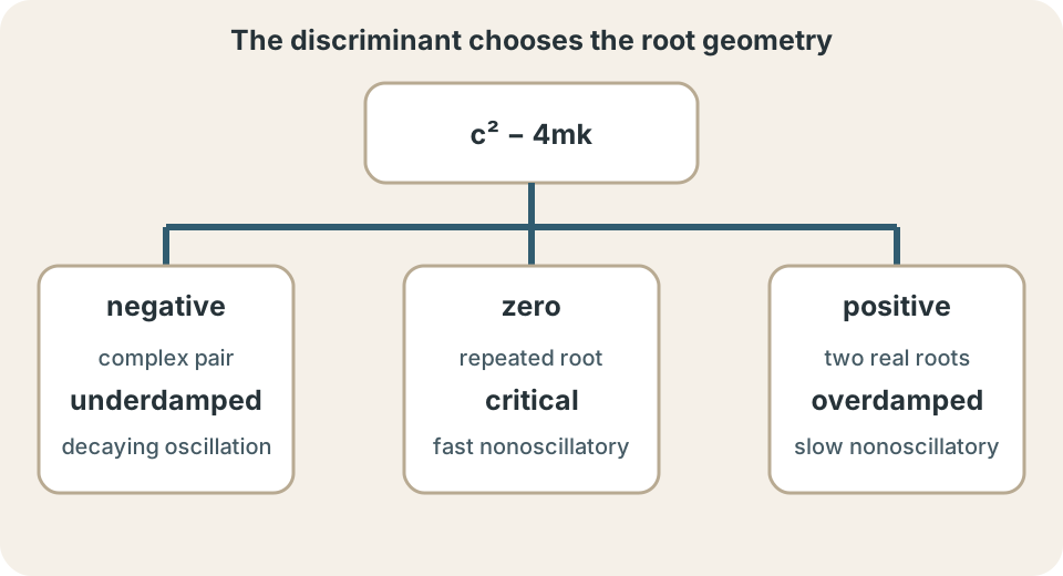
The quadratic formula gives $r=\frac{-c\pm\sqrt{c^2-4mk}}{2m}$. The horizontal fraction divides the entire numerator by $2m$. The expression under the square root is the discriminant. Its sign determines whether roots are real and distinct, repeated, or complex conjugates. Those root types become the damping regimes.

Initial conditions do not change the roots. They select coefficients multiplying the fundamental solutions. A system can be underdamped even if one special initial condition produces no visible motion. Regime is a property of $m$, $c$, and $k$. Particular trajectory is a property of coefficients plus initial state.

Normalize the equation

Divide $mx''+cx'+kx=0$ by positive mass $m$. The result is $x''+\frac{c}{m}x'+\frac{k}{m}x=0$. Define undamped natural angular frequency $\omega_n=\sqrt{\frac{k}{m}}$. It has unit $\mathrm{\frac{rad}{s}}$. The subscript $n$ means natural.

Define damping ratio $\zeta=\frac{c}{2\sqrt{mk}}$. Greek letter $\zeta$ is pronounced zeta. Numerator and denominator both have unit $\mathrm{\frac{kg}{s}}$, so the ratio is dimensionless. Then $\frac{c}{m}=2\zeta\omega_n$. The normalized equation becomes $x''+2\zeta\omega_nx'+\omega_n^2x=0$.

Nondimensional ratio $\zeta$ compares actual damping with critical damping. Systems with different masses and stiffnesses can share the same normalized response shape. Natural frequency sets the time scale. Damping ratio sets the qualitative regime. This separation supports design comparisons.

Underdamping produces decaying oscillation

When $c^2<4mk$, the roots are complex. In ratio form, this means $0<\zeta<1$. Write roots as $r=-\zeta\omega_n\pm i\omega_d$. Damped angular frequency is $\omega_d=\omega_n\sqrt{1-\zeta^2}$. It is smaller than $\omega_n$.

The real solution is $x(t)=e^{-\zeta\omega_nt}[C_1\cos(\omega_dt)+C_2\sin(\omega_dt)]$. The exponential factor is the decay envelope. The sine and cosine factors create crossings and oscillations. Constants $C_1$ and $C_2$ come from initial displacement and velocity. Reading the product this way separates shrinking magnitude from repeated motion.

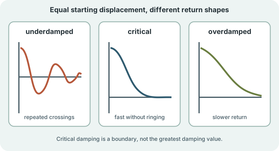
The response crosses equilibrium repeatedly unless a degenerate zero-amplitude condition removes motion. Peak magnitudes shrink approximately along $\pm Ae^{-\zeta\omega_nt}$. The oscillation period is $T_d=\frac{2\pi}{\omega_d}$. Damping both reduces amplitude and slightly lowers frequency. A graph should therefore show narrowing envelopes and widening periods relative to the undamped case.

Critical damping is the boundary

When $c^2=4mk$, the characteristic root repeats. In ratio form, $\zeta=1$. The root is $r=-\omega_n$. Two independent solutions are $e^{-\omega_nt}$ and $te^{-\omega_nt}$. Therefore $x(t)=(C_1+C_2t)e^{-\omega_nt}$.

Critical damping returns toward equilibrium without sustained oscillation. It is often described as the fastest nonoscillatory response under comparable initial and model conditions. That phrase needs context because particular initial conditions affect settling and crossing. It does not mean infinite or maximum damping. It is the boundary value.

Door closers and measurement instruments may be designed near critical damping. Too little damping creates unwanted ringing. Too much damping makes response sluggish. Critical design balances speed and overshoot. Real nonlinear devices may only approximate the linear ideal.

Overdamping uses two real decay rates

When $c^2>4mk$, roots are distinct, real, and negative for positive coefficients. Ratio satisfies $\zeta>1$. The solution is $x(t)=C_1e^{r_1t}+C_2e^{r_2t}$. Both modes decay. One root is closer to zero and becomes the slow mode.

An overdamped response does not repeatedly oscillate. It usually returns more slowly than a critically damped system with the same $m$ and $k$. Increasing damping can make the slow root even closer to zero. Strong resistance inhibits motion. More damping can therefore lengthen settling time.

Particular initial conditions can allow one equilibrium crossing. “Nonoscillatory” means no repeated alternating crossings. The sum of two exponentials can change sign once. Inspect coefficients before claiming monotone position. Energy still decreases under positive viscous damping.

Worked coefficient example

Consider $x''+4x'+13x=0$ with time in seconds. It corresponds to normalized mass $m=1$, damping $c=4\,\mathrm{\frac{kg}{s}}$, and stiffness $k=13\,\mathrm{\frac{N}{m}}$ under compatible units. The characteristic equation is $r^2+4r+13=0$. Its discriminant is $16-52=-36$. The system is underdamped.

Roots are $r=\frac{-4\pm\sqrt{-36}}{2}=-2\pm3i\,\mathrm{\frac{1}{s}}$. The real part gives decay rate $2\,\mathrm{\frac{1}{s}}$. The imaginary magnitude gives damped angular frequency $3\,\mathrm{\frac{rad}{s}}$. Thus $x=e^{-2t}(C_1\cos3t+C_2\sin3t)$ when units are understood in the arguments. Exponents and trigonometric arguments are dimensionless.

Natural frequency is $\omega_n=\sqrt{13}\,\mathrm{\frac{rad}{s}}$. Damping ratio is $\zeta=\frac{2}{\sqrt{13}}\approx0.555$. Check $\omega_d=\omega_n\sqrt{1-\zeta^2}=3\,\mathrm{\frac{rad}{s}}$. The independent calculations agree. This closes the coefficient-root-parameter loop.

Initial conditions select constants

Suppose $x(0)=x_0$ and $x'(0)=v_0$. In the underdamped form, evaluating at zero gives $C_1=x_0$. Differentiate the full product before setting $t=0$. The result gives $v_0=-\zeta\omega_nC_1+\omega_dC_2$. Therefore $C_2=\frac{v_0+\zeta\omega_nx_0}{\omega_d}$.

Position $x_0$ has unit metres and velocity $v_0$ has $\mathrm{\frac{m}{s}}$. Numerator in $C_2$ has velocity units because $\omega_nx_0$ is $\mathrm{\frac{m}{s}}$. Dividing by $\omega_d$ leaves metres. Both constants then match displacement units. Dimensional consistency verifies the expression.

Different initial conditions can suppress one overdamped mode or shift the phase of an underdamped response. They do not change $\zeta$ or root locations. A zero initial displacement with nonzero velocity still excites motion. State requires two initial values because the ODE is second order. These two values specify one point in the position–velocity state plane.

Amplitude–phase form

The combination $C_1\cos(\omega_dt)+C_2\sin(\omega_dt)$ can be rewritten $A\cos(\omega_dt-\phi)$. Amplitude constant is $A=\sqrt{C_1^2+C_2^2}$. Phase satisfies relationships such as $C_1=A\cos\phi$ and $C_2=A\sin\phi$. Quadrant-aware angle selection matters. Using a two-argument inverse tangent prevents an incorrect phase quadrant.

The full displacement is $x(t)=Ae^{-\zeta\omega_nt}\cos(\omega_dt-\phi)$. The factor $A$ is an initial envelope scale, not a constant oscillation amplitude. Instantaneous envelope magnitude decreases exponentially. Phase $\phi$ shifts peak timing. Decay rate and frequency remain system properties.

Amplitude–phase form is convenient for fitting and interpretation. Sine–cosine form is convenient for applying initial conditions algebraically. They describe the same solution. Converting forms should preserve units and quadrants. Representation choice changes convenience, not physics.

Energy decreases monotonically

Mechanical energy is $E=\frac{1}{2}mx'^2+\frac{1}{2}kx^2$. The first term is kinetic energy and the second spring potential energy. Both have unit joules. Differentiate with respect to time. Product and chain rules are required.

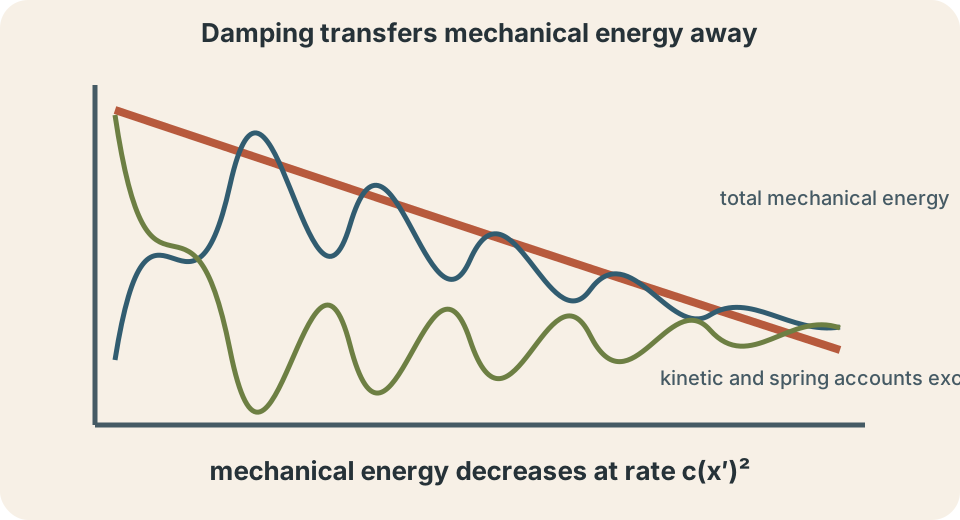
The derivative is $\frac{dE}{dt}=mx'x''+kxx'=x'(mx''+kx)$. From the motion equation, $mx''+kx=-cx'$. Substitute to obtain $\frac{dE}{dt}=-c(x')^2\leq0$. Positive damping makes energy nonincreasing. The inequality is an energy argument for stability rather than merely a feature of the plotted solution.

Position can oscillate while total mechanical energy decreases. At turning points, velocity is zero and instantaneous dissipation rate is zero. Between them, moving damper removes energy. Lost mechanical energy becomes internal energy in the damper and surroundings. Energy is transferred or transformed rather than destroyed.

Energy decay and amplitude decay differ

For light damping, displacement envelope decays as $e^{-\zeta\omega_nt}$. Mechanical energy is approximately proportional to amplitude squared. Its envelope therefore decays roughly as $e^{-2\zeta\omega_nt}$. Energy decay rate is twice the amplitude exponent. These are related but distinct measurements.

The time constant for amplitude is $\tau=\frac{1}{\zeta\omega_n}=\frac{2m}{c}$. After one time constant, the envelope falls by factor $e^{-1}\approx0.368$. After three, it is about $0.050$ of its initial scale. A tolerance determines practical settling. Time constants translate an abstract exponent into an observable decay schedule.

Exact total energy contains oscillatory exchange between kinetic and potential accounts. Its derivative never becomes positive under this model. A smooth exponential may approximate the envelope rather than each instant. State whether a fit targets peaks, root-mean-square amplitude, or energy. Measurement definition matters.

Logarithmic decrement estimates damping

For an underdamped response, successive same-direction peaks are separated by one damped period. If peak magnitudes are $x_n$ and $x_{n+1}$, logarithmic decrement is $\delta=\ln\left(\frac{x_n}{x_{n+1}}\right)$. The ratio is dimensionless. Positive $\delta$ indicates decay. The same peak convention must be used.

Under the ideal model, $\delta=\frac{2\pi\zeta}{\sqrt{1-\zeta^2}}$. Solving gives $\zeta=\frac{\delta}{\sqrt{4\pi^2+\delta^2}}$. Multiple cycles can reduce measurement error: $\delta=\frac{1}{N}\ln\left(\frac{x_n}{x_{n+N}}\right)$. Here $N$ is number of periods. Peak signs are handled through magnitudes.

Noise, nonlinear damping, and changing frequency can bias the estimate. Plotting logarithm of peak magnitude against time should give an approximately straight line for exponential decay. Its slope estimates $-\zeta\omega_n$. Residuals test the model. One pair of peaks provides weaker evidence than many.

Quality factor for light damping

Quality factor $Q$ summarizes weak damping in oscillators. One common relation is $Q=\frac{1}{2\zeta}$ for a lightly damped second-order system. Larger $Q$ means slower relative energy loss and sharper resonance. Smaller $Q$ means stronger damping. The exact interpretation depends on convention and system.

Another definition relates stored energy to energy lost per radian or cycle. Under weak damping, these definitions align closely. Outside that regime, formulas must be chosen carefully. State the definition being used. Do not confuse quality factor with heat transfer $Q$ from thermodynamics.

An instrument may need high $Q$ for narrow frequency selectivity. A suspension may need moderate damping for rapid settling. A resonator and a door closer have different objectives. Dimensionless metrics support comparison. Design context determines desirable value.

Settling time and overshoot

Settling time is the time after which response remains within a specified band around equilibrium. The band might be $2\%$ or $5\%$ of a reference amplitude. Without the band, “settled” is ambiguous. Underdamped response may enter and leave the band before final entry. Envelope estimates provide conservative timing.

For an underdamped normalized second-order response, envelope $Ae^{-\zeta\omega_nt}$ gives approximate settling condition. Solve $e^{-\zeta\omega_nt}\leq\varepsilon$ to obtain $t\geq\frac{-\ln\varepsilon}{\zeta\omega_n}$. The tolerance $\varepsilon$ is dimensionless. Initial scaling and response type can modify the practical result. Report the chosen tolerance whenever a numerical settling time is quoted.

Critical damping often minimizes settling without oscillatory overshoot for standard step-response criteria. Free response and forced step response are not identical tasks. Overdamping removes ringing but can be slow. Underdamping can settle quickly in envelope while crossing repeatedly. Specify the performance metric.

Free response differs from forced response

The free equation has zero right side. A driven system has $mx''+cx'+kx=F(t)$. External force $F(t)$ injects energy. The total response combines transient motion and a particular forced response. Damping controls both.

For sinusoidal driving, long-term response can persist despite damping because the driver replaces dissipated energy. Resonance frequency and amplitude depend on damping. The free transient still decays according to characteristic roots. Eventually the forced steady state can dominate. This distinction prevents confusing dissipation with the absence of sustained motion.

Do not say damping always makes displacement approach zero. That is true for stable unforced motion around zero equilibrium. Constant forcing can shift equilibrium. Periodic forcing can sustain oscillation. Boundary conditions and input determine the target behavior.

Phase-space interpretation

Define velocity $v=x'$. The second-order ODE becomes system $x'=v$ and $v'=-\frac{k}{m}x-\frac{c}{m}v$. A state is point $(x,v)$ in phase space. Equilibrium is $(0,0)$. Trajectories show position and velocity together.

Underdamped trajectories spiral toward the origin. Critical and overdamped trajectories approach without spiraling. The linear-system eigenvalues are the characteristic roots already derived. Complex roots produce rotation with decay. Real roots produce nonoscillatory modal approach.

Phase space clarifies why position alone can cross zero while the state is not at equilibrium. At $x=0$ with $v\ne0$, motion continues. Equilibrium requires both coordinates zero. The energy function forms shrinking contours under damping. Geometry unifies ODE and mechanics.

Parameter changes and design

Increasing stiffness raises $\omega_n=\sqrt{\frac{k}{m}}$ if mass is fixed. It also changes damping ratio because $\zeta=\frac{c}{2\sqrt{mk}}$. Increasing $k$ can lower $\zeta$ for fixed $c$. The response may become faster and relatively less damped. Parameters interact.

Increasing mass lowers natural frequency. It also lowers damping ratio for fixed $c$ and $k$. A heavier system can become more oscillatory. To preserve $\zeta$, damping coefficient must scale with $\sqrt{mk}$. Dimensional groups guide similarity.

Critical damping coefficient is $c_c=2\sqrt{mk}$. Actual ratio is $\zeta=\frac{c}{c_c}$. This makes the word “critical” concrete. It is a finite boundary value, not maximum damping. Design can target a ratio above, below, or near one.

Experimental estimation and uncertainty

Displacement can be measured with a position sensor or video tracking. Sampling rate must resolve the damped period. Sensor offset affects equilibrium estimate. Noise affects peaks and numerical derivatives. Calibration supplies physical units.

Estimate $\omega_d$ from time between like peaks. Estimate decay rate from a fitted line to logarithmic peak amplitudes. Then recover $\omega_n=\sqrt{\omega_d^2+(\zeta\omega_n)^2}$ through a consistent parameterization. Nonlinear fitting can estimate all parameters together. Residuals should be inspected.

Uncertainty comes from timing, position scale, noise, model mismatch, and parameter correlation. Reporting many calculator digits does not remove it. Repeated trials estimate variability. Independent mass or stiffness measurements can constrain the fit. Every inferred parameter should include units and method.

Common misconceptions and repairs

One misconception says critical damping is maximum damping. It is the boundary between oscillatory and nonoscillatory roots. Overdamped systems have more damping. They can respond more slowly. Use discriminant or $\zeta$ to classify.

Another misconception says overdamped motion can never cross equilibrium. It cannot repeatedly oscillate, but a particular sum of two decaying exponentials may cross once. Initial velocity matters. Examine constants or simulate. Avoid replacing “nonoscillatory” with “monotone” automatically.

A third misconception confuses $\omega_n$ with $\omega_d$. Natural frequency belongs to the undamped parameter combination. Damped frequency is lower when $0<\zeta<1$. Decay rate is a separate real-root component. Read each part of $-\zeta\omega_n\pm i\omega_d$.

A reliable analysis routine

Write the equation with units and confirm positive physical coefficients. Divide by mass. Calculate $\omega_n$ and $\zeta$. Alternatively compute discriminant $c^2-4mk$. Classify the roots before solving constants.

Write the correct regime solution. Apply both initial conditions. Verify units in exponential and trigonometric arguments. Substitute the solution or roots back into the ODE. Interpret decay rate, oscillation frequency, and settling behavior separately.

Use the energy derivative to check physical damping. Compare model predictions with observed peaks and periods. State whether motion is free or forced. Name assumptions such as linear stiffness and viscous damping. Finish with a response interpretation tied to the application.

Practice and connection forward

For $m=1.00\,\mathrm{kg}$, $k=16.0\,\mathrm{\frac{N}{m}}$, and $c=4.00\,\mathrm{\frac{kg}{s}}$, natural frequency is $4.00\,\mathrm{\frac{rad}{s}}$. Critical coefficient is $8.00\,\mathrm{\frac{kg}{s}}$. Thus $\zeta=\frac{4.00}{8.00}=0.500$. The system is underdamped. The ratio predicts oscillation before any constants are calculated.

If $c$ increases to $8.00\,\mathrm{\frac{kg}{s}}$, it becomes critically damped. If $c=12.0\,\mathrm{\frac{kg}{s}}$, ratio is $1.50$ and it is overdamped. Mass and stiffness stay fixed. Only damping regime changes. Comparing these cases isolates the causal role of the damping coefficient.

Without looking back, derive the characteristic equation and energy-loss equation. Explain why stronger overdamping can slow response. Distinguish $\omega_n$, $\omega_d$, and decay rate. Forced-oscillation analysis will add a continuing energy input. Phase-plane analysis will interpret the same roots geometrically.