Systems of ODEs Track Interacting Quantities

Real systems rarely contain one changing quantity in isolation. Predator and prey populations interact, chemical species react, temperature moves between connected bodies, and position and velocity evolve together. A system of ordinary differential equations assigns a rate law to every state variable simultaneously. Coupling means the current value of one variable can influence the rate of another. The resulting vector viewpoint reveals trajectories, equilibria, stability, oscillation, and collective behavior that one scalar equation cannot express alone.

Learning objectives and the complete-state viewpoint

By the end of this article, you will write coupled rate laws in component and vector form and interpret every term with units. You will convert higher-order scalar equations into first-order systems. You will construct and read phase-plane vector fields, nullclines, equilibria, and trajectories. You will solve simple linear systems using eigenvalues and eigenvectors and classify local stability. You will also linearize nonlinear systems, apply numerical methods, and verify models through invariants, bounds, and representation checks.

The central idea is the state. A state vector contains enough information at one time to determine all rates under the model. Position alone is not a complete state for second-order motion because velocity is also needed. Two population sizes may form a complete state for a two-species model. Choosing state variables is therefore a modeling decision.

Once the state is chosen, the differential equation defines a vector field on state space. At each state, the field supplies a direction and speed of change. A solution trajectory follows those arrows as time advances. The same point cannot generally have two different future directions under a single-valued autonomous model. Geometry and algebra describe one evolving object.

Write coupled equations component by component

A two-state system has the form $x'=f(t,x,y)$ and $y'=g(t,x,y)$. The primes denote derivatives with respect to the common independent variable, usually time. The first rate may depend on both current states, and so may the second. That cross-dependence creates coupling. If each equation depends only on its own variable, the system is uncoupled and can be solved separately.

Consider two tanks exchanging dissolved material. Let $x(t)$ and $y(t)$ be masses in kilograms. A transfer rate from tank one to tank two may be $k_{12}x$, while reverse transfer may be $k_{21}y$. Then $x'=-k_{12}x+k_{21}y$ and $y'=k_{12}x-k_{21}y$. Each transfer appears with opposite signs because material leaving one tank enters the other.

Units verify the construction. If time is hours, coefficients $k_{12}$ and $k_{21}$ have units $\frac{1}{\mathrm h}$. Multiplying by kilograms gives $\frac{\mathrm{kg}}{\mathrm h}$, matching $x'$ and $y'$. A term with incompatible units cannot be added. Dimensional consistency catches many coupling errors.

Compress the system into vector form

Define state vector $\mathbf x=(x_1,x_2,\ldots,x_n)^T$. A general first-order system is $\mathbf x'=\mathbf f(t,\mathbf x)$. The bold symbols denote vectors, and the superscript $T$ indicates a column orientation. Function $\mathbf f$ returns one rate component for every state component. The vector equation is shorthand for all scalar equations together.

An autonomous system has no explicit time dependence and is written $\mathbf x'=\mathbf f(\mathbf x)$. Time still changes along a solution, but the rate assigned to a state is the same whenever that state is visited. A nonautonomous system includes explicit forcing or changing coefficients through $t$. The distinction matters for phase-space geometry. Autonomous trajectories cannot cross under uniqueness conditions because the crossing state would require two directions.

For a linear autonomous system, $\mathbf x'=A\mathbf x$. Matrix entry $a_{ij}$ measures how state component $x_j$ contributes to rate component $x_i$. Rows correspond to rate equations, while columns correspond to state influences. Matrix multiplication builds each rate as a linear combination of current states. The matrix is a map from state units to rate units.

Convert higher-order equations into first-order systems

Any scalar equation of order $n$ can be represented as $n$ first-order equations by introducing variables for successive derivatives. For $y''+cy'+ky=0$, define $x_1=y$ and $x_2=y'$. Then $x_1'=x_2$. Rearranging the original equation gives $x_2'=y''=-kx_1-cx_2$. Together these equations preserve the original dynamics.

The state $(x_1,x_2)$ represents position-like quantity and its rate. Initial conditions $y(t_0)=y_0$ and $y'(t_0)=v_0$ become $\mathbf x(t_0)=(y_0,v_0)^T$. A numerical solver for first-order systems can now integrate the second-order problem. The conversion changes representation rather than physical content. It also exposes phase-plane behavior.

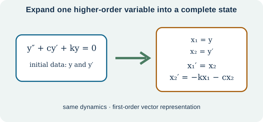
For an $n$th-order equation, use $x_1=y$, $x_2=y'$, through $x_n=y^{(n-1)}$. The first $n-1$ equations shift derivatives upward. The final equation comes from solving the original equation for $y^{(n)}$. This companion-system form is systematic. State units can differ across components because derivatives carry different powers of time.

Read a phase plane as state space

For a two-dimensional autonomous system, the phase plane uses $x$ and $y$ as axes. A point represents the complete state at one time rather than a location in physical space unless the states themselves are positions. The vector $(f(x,y),g(x,y))$ is drawn at that point. Its direction shows instantaneous state change. Its magnitude reflects speed through state space under the axis units.

A trajectory is a curve traced by one solution as time changes. Arrowheads indicate forward-time direction. Closely spaced time marks mean slower travel and widely spaced marks mean faster travel, if marks use equal time intervals. The curve alone does not reveal speed. A phase portrait combines representative trajectories, equilibria, and field information.

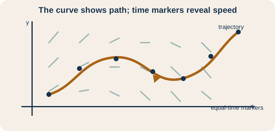
Time is implicit in a phase-plane plot. A separate time-series plot shows each component against time and can reveal timing more directly. The two representations complement one another. Closed loops in phase space correspond to periodic state repetition under suitable conditions. Similar-looking projections can have different timing.

Find nullclines and equilibria

An $x$-nullcline is the set where $x'=f(x,y)=0$. Along it, the vector field has no horizontal component. A $y$-nullcline is the set where $y'=g(x,y)=0$. Along it, the field has no vertical component. Nullclines divide the plane into regions with consistent sign patterns.

An equilibrium is a state $\mathbf x^*$ satisfying $\mathbf f(\mathbf x^*)=\mathbf0$. In two dimensions, equilibria occur at intersections of both nullclines. Starting exactly at an equilibrium produces a constant solution. Equilibria organize nearby trajectories. They should be found before divisions that could remove zero factors.

For $x'=x(1-y)$ and $y'=y(x-1)$, $x$-nullclines are $x=0$ and $y=1$. The $y$-nullclines are $y=0$ and $x=1$. Their intersections include $(0,0)$ and $(1,1)$. Sign analysis in surrounding regions predicts directional flow. Algebra supplies boundaries while geometry assembles the portrait.

Use sign regions before solving formulas

Between nullclines, determine signs of $x'$ and $y'$. The pair $(+,+)$ points right and up, $(+,-)$ points right and down, $(-,+)$ points left and up, and $(-,-)$ points left and down. One test point in each connected region usually determines signs when formulas are continuous. This creates a qualitative vector field. Exact arrow angles require evaluating magnitudes as well.

Sign analysis can reveal invariant regions. If vectors along a boundary point inward or tangent, trajectories may remain inside. Population models often require $x\ge0$ and $y\ge0$. Rate laws should preserve that nonnegative quadrant. A vector pointing into negative population values at a boundary signals a modeling or interpretation problem.

Qualitative information can rule out numerical artifacts. A computed trajectory crossing a uniqueness-protected equilibrium line may indicate excessive step size or coding error. A solution leaving a positively invariant region may violate model structure. Phase geometry therefore supports verification even when no closed form exists. Do not wait for an explicit formula before reasoning.

Solve a diagonal linear system

Consider $x'=-x$ and $y'=2y$. The equations are uncoupled, so $x=C_1e^{-t}$ and $y=C_2e^{2t}$. The $x$ component decays forward in time, while the $y$ component grows unless $C_2=0$. The origin is an equilibrium. The coordinate axes are invariant because starting with one component zero keeps it zero.

Matrix form is $\mathbf x'=\begin{bmatrix}-1&0\\0&2\end{bmatrix}\mathbf x$. Eigenvalues are $-1$ and $2$, with eigenvectors along coordinate axes. One eigendirection is stable and one is unstable. Generic trajectories approach the origin in one time direction and leave in the other. This equilibrium is a saddle.

Eliminating time gives a trajectory relation when constants are nonzero. From $x=C_1e^{-t}$, one obtains $e^t=C_1/x$ in an appropriate sign region. Substituting into $y=C_2e^{2t}$ gives $y=Cx^{-2}$ for a constant $C$. These curves show paths but not temporal speed. The explicit time solution retains more information.

Build linear solutions from eigenmodes

For $\mathbf x'=A\mathbf x$, suppose $A\mathbf v=\lambda\mathbf v$. Then $\mathbf x(t)=e^{\lambda t}\mathbf v$ satisfies the system because $\mathbf x'=\lambda e^{\lambda t}\mathbf v$ and $A\mathbf x=e^{\lambda t}A\mathbf v$. The eigenvector supplies an invariant direction. The eigenvalue supplies growth, decay, or oscillatory rate. This pair forms a mode.

If $A$ has enough independent eigenvectors, the general solution is a linear combination $\mathbf x(t)=\sum_j C_je^{\lambda_jt}\mathbf v_j$. Constants are determined by the initial state. Each mode evolves independently under the linear system. Long-term behavior is often dominated by the eigenvalue with largest real part. Initial conditions can remove a mode only when its coefficient is exactly zero.

Repeated eigenvalues may lack enough independent eigenvectors. Generalized eigenvectors and polynomial factors in time are then needed. Complex eigenvalues occur in conjugate pairs for real matrices and produce real sine-cosine combinations. Matrix exponentials provide the unified solution $\mathbf x(t)=e^{At}\mathbf x(0)$. Eigenmode reasoning explains the structure of that exponential.

Classify two-dimensional linear equilibria

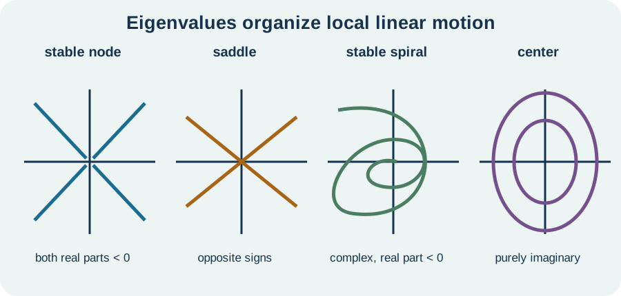
If both eigenvalues have negative real parts, the origin is asymptotically stable. Two negative real eigenvalues typically produce a stable node, while a complex pair with negative real part produces a stable spiral. If both real parts are positive, the equilibrium is unstable. Opposite-sign real eigenvalues produce a saddle. Eigenvalue signs organize local growth and decay directions.

Purely imaginary eigenvalues in a linear system produce a center under appropriate diagonalizability, with closed orbits and neutral stability. Repeated zero or zero-real-part cases require care. For nonlinear systems, linearization with eigenvalues on the imaginary axis is inconclusive. Higher-order terms can create stability or instability. Classification rules have assumptions.

Trace and determinant summarize a $2\times2$ matrix. Eigenvalues satisfy $\lambda^2-\tau\lambda+\Delta=0$, where $\tau=\operatorname{tr}(A)$ and $\Delta=\det(A)$. Determinant sign identifies saddles when negative, while trace influences real-part sign. The discriminant $\tau^2-4\Delta$ separates real and complex roots. A trace-determinant plane compresses classification but should not replace eigenvalue meaning.

Linearize a nonlinear system near equilibrium

For nonlinear autonomous system $\mathbf x'=\mathbf f(\mathbf x)$, let $\mathbf x^*$ be an equilibrium. Write a small perturbation $\mathbf u=\mathbf x-\mathbf x^*$. A first-order Taylor approximation gives $\mathbf u'\approx J(\mathbf x^*)\mathbf u$. The Jacobian has entries $J_{ij}=\frac{\partial f_i}{\partial x_j}$. It is the local matrix of rate sensitivities.

If no Jacobian eigenvalue has zero real part, the linearization often correctly predicts local stability type under standard theorems. Negative real parts imply local attraction, while any positive real part implies instability. The result is local because the Taylor approximation is valid near equilibrium. Distant trajectories may encounter other equilibria, invariant sets, or nonlinear behavior. A local classification is not a global portrait.

When eigenvalues have zero real parts, linearization may be inconclusive. Nonlinear terms omitted from the Jacobian can determine behavior. Center manifolds, Lyapunov functions, normal forms, or direct nonlinear analysis may be needed. Do not force a node-or-spiral label from insufficient evidence. Inconclusive is a valid mathematical conclusion.

Model interacting populations

A predator-prey model may use prey $x$ and predator $y$. A classical form is $x'=ax-bxy$ and $y'=-cy+dxy$, with positive parameters. Prey grow at rate $ax$ without predators and are removed through encounters $bxy$. Predators decline at rate $cy$ without prey and gain through encounters $dxy$. Each term has a mechanistic interpretation.

Units constrain parameters. If populations are counts and time is days, $a$ and $c$ have units $\frac{1}{\mathrm{day}}$. Since $xy$ has squared-count units, $b$ and $d$ must convert encounter products into count per day. Depending on how populations are normalized, coefficient units change. Model documentation should define state scales.

The model is an idealization. Unlimited prey growth, mass-action encounters, constant parameters, and no age structure may be unrealistic. Its closed-orbit behavior is not a universal law of ecosystems. Adding carrying capacity, saturation, seasons, or spatial structure changes dynamics. Mathematical elegance does not guarantee ecological adequacy.

Build compartment and conservation models

Compartment models represent material moving among connected stores. Each state records amount in one compartment. Transfer from compartment $j$ to $i$ appears positively in equation $i$ and negatively in equation $j$. External inputs and outputs break internal conservation. A diagram of arrows can be translated systematically into rate equations.

For two closed compartments with rates $k_{12}x$ and $k_{21}y$, adding equations gives $(x+y)'=0$. Therefore total amount $x+y$ is conserved. The vector $(1,1)$ defines a left-null relationship with the transfer matrix. Conservation provides an invariant. Numerical solutions should preserve it within expected error.

If material leaves the system at rate $ky$, then $(x+y)'=-ky$. Total amount is no longer constant but decreases when $y>0$. This balance equation checks signs and units. Conservation laws can reduce system dimension or constrain trajectories. They also connect differential equations to physical accounting.

Use nullclines in chemical and biological networks

Nullclines show where one rate vanishes, not where the entire state stops. A trajectory can cross an $x$-nullcline vertically because $x'=0$ while $y'$ remains nonzero. Similarly, it can cross a $y$-nullcline horizontally. Only an intersection of all relevant nullclines is an equilibrium. This directional interpretation prevents a common plotting mistake.

In a reaction network, nullclines can represent production-loss balance for one species. Their intersections identify steady states. Multiple intersections can indicate multiple steady regimes. Stability analysis determines which are attracting. Parameters can move nullclines and create or destroy equilibria.

Bifurcation occurs when qualitative dynamics change as a parameter passes a threshold. Equilibria may exchange stability, appear, disappear, or generate oscillations. Nullcline geometry can make these changes visible. A parameter sweep should track both equilibrium locations and eigenvalues. One fitted parameter set cannot reveal the full regime structure.

Integrate systems numerically

Euler’s method generalizes to vectors as $\mathbf x_{n+1}=\mathbf x_n+h\mathbf f(t_n,\mathbf x_n)$. The step size $h$ has independent-variable units. Multiplying each rate component by $h$ produces a compatible state change. Every component updates from the same current state in forward Euler. Sequentially updating one component before evaluating another would implement a different method.

Higher-order Runge–Kutta methods evaluate several intermediate field values per step. Adaptive solvers adjust step size using error estimates. Stiff systems may require implicit methods for stability. Solver choice depends on timescales, accuracy needs, events, and conservation structure. Default settings should not be accepted blindly.

Numerical verification includes step refinement, invariant checks, nonnegativity, equilibrium behavior, and comparison with solvable cases. Plot both time series and phase trajectories. Record tolerances and method. A smooth graph can still be inaccurate. Numerical results require evidence of convergence.

Preserve units in mixed-state systems

State components can have different units. Position may be meters while velocity is meters per second. Matrix entries then carry units that map each state into each rate equation. In $x_1'=x_2$, the coefficient multiplying velocity is dimensionless because both sides have meters per second. In $x_2'=-kx_1-cx_2$, coefficients supply appropriate inverse-time powers.

Adding mixed-unit components inside a norm requires scaling choices. A distance of one meter and velocity of one meter per second cannot be compared numerically without reference scales. Error tolerances for numerical solvers often use component-specific absolute and relative scales. Phase-plane visual angles also depend on axis units. Coordinate geometry must respect dimensional meaning.

Nondimensionalization introduces reference scales to produce unit-free variables and parameters. It can reduce parameter count and reveal dominant ratios. The process must be reversible and documented. Dimensionless models improve comparison but do not erase physical interpretation. Results must return to original units for application.

Verify existence, uniqueness, and domain behavior

For $\mathbf x'=\mathbf f(t,\mathbf x)$, continuity of $\mathbf f$ supports local existence under common theorems. Local Lipschitz behavior in the state supports uniqueness. A continuously differentiable vector field is locally Lipschitz. These are sufficient conditions rather than necessary ones. Singularities and discontinuities require separate analysis.

Uniqueness explains why autonomous trajectories cannot cross at an ordinary point. A crossing would assign two distinct solution paths to the same state. Curves may appear to intersect in a projection from higher dimensions or at different times in nonautonomous extended space. The complete state representation matters. Phase portraits assume enough state variables to make evolution single-valued.

Local existence does not guarantee a solution for all time. Components can diverge in finite time or reach a model boundary. Rate laws may be undefined at zero or negative states. Numerical solvers can step outside the domain even when the true solution remains inside. State constraints and maximal intervals must be monitored.

Diagnose common misconceptions

A phase-plane trajectory is not a graph of one state against time. Time is implicit, and path slope is not temporal speed. Use arrows and time markers to recover direction and speed information. Another mistake treats a nullcline as an equilibrium curve. Check all rate components simultaneously.

Eigenvalues classify linear systems globally but nonlinear systems only locally near an equilibrium under appropriate conditions. Zero real parts make linearization inconclusive. A stable equilibrium does not imply every initial state approaches it. Basins of attraction can be limited by separatrices or other invariant sets. State the scope of each conclusion.

Modeling mistakes include missing transfer signs, incompatible units, and impossible negative states. Draw a flow diagram and perform total-balance checks. Numerical mistakes include asynchronous component updates and untested step sizes. Verify against invariants and alternative solvers. Systems reward organized bookkeeping.

Practice vector form, equilibria, and stability

Convert $y''+3y'+2y=0$ into a first-order system with state $(y,v)$. Write its matrix, units, equilibrium, eigenvalues, and general qualitative behavior. Explain why two initial conditions are needed. Identify whether the origin is stable. Connect characteristic roots to matrix eigenvalues.

For $x'=-2x+y$ and $y'=x-2y$, find the equilibrium and eigenvalues. Determine eigenvector directions and classify the origin. Predict long-term behavior for any initial state. Verify that the line $x=y$ is invariant. State which mode decays more slowly.

For closed transfer system $x'=-0.3x+0.1y$ and $y'=0.3x-0.1y$ in kilograms per hour, verify total conservation. Find the equilibrium relationship under fixed total $M$. Interpret coefficients and units. Explain how a numerical solution could be checked. Identify one zero eigenvalue’s physical meaning.

Solutions and reasoning

Set $x_1=y$ and $x_2=v=y'$. Then $\mathbf x'=\begin{bmatrix}0&1\\-2&-3\end{bmatrix}\mathbf x$. The origin is equilibrium, and eigenvalues satisfy $\lambda^2+3\lambda+2=0$, giving $-1$ and $-2$. Both are negative, so the origin is asymptotically stable. Position and velocity initial values specify the complete state. The slower negative-one mode dominates long-term decay.

Matrix is $\begin{bmatrix}-2&1\\1&-2\end{bmatrix}$. Eigenvalues are $-1$ along vector $(1,1)$ and $-3$ along $(1,-1)$. Both are negative, so the origin is a stable node. Every solution approaches zero. The line $x=y$ is invariant because states on it have rates proportional to $(1,1)$. The negative-one mode decays more slowly.

Adding transfer equations gives $(x+y)'=0$, so total $M=x+y$ is conserved in kilograms. At equilibrium, $0.3x=0.1y$, so $y=3x$. Together with $x+y=M$, this gives $x=M/4$ and $y=3M/4$. Coefficients have units inverse hours. The zero eigenvalue reflects the continuum of equilibria across different conserved totals, while each fixed total selects one. A numerical solution should preserve total mass and approach the appropriate equilibrium.

Carry systems thinking into broader dynamics

Systems of ODEs provide one language for interacting states across mechanics, chemistry, biology, circuits, and control. Vector fields express local rules, phase planes organize trajectories, nullclines locate directional boundaries, and equilibria anchor behavior. Eigenvalues decompose linear motion into modes. Jacobians extend that insight locally to nonlinear systems. Together, these representations connect an equation’s local rates to the system’s observable long-term behavior.

Higher-dimensional systems use the same ideas but require projections, numerical tools, and additional theory. Bifurcations track parameter-driven qualitative change. Lyapunov functions can prove stability without explicit solutions. Conservation laws and symmetries reduce complexity. Computational models reveal patterns but require verification.

When building or reading a system, define complete states, units, couplings, inputs, outputs, and domain. Check balances and invariants before solving. Combine time series, phase portraits, eigenvalue analysis, and numerical refinement. A trustworthy model explains how component interactions produce the collective trajectory. That explanation, rather than a collection of disconnected calculations, is the central goal of systems analysis.