Ordinary Differential Equations Describe Evolving Systems

Many scientific laws do not state a quantity directly. They state how that quantity changes in response to its present state, time, or external inputs. An ordinary differential equation, abbreviated ODE, connects an unknown function of one independent variable to one or more of its derivatives. The equation supplies a local rule, while initial or boundary information selects a trajectory that follows that rule. Understanding ODEs therefore means learning to move between rates, functions, geometry, approximation, and physical interpretation.

Establish the foundational questions

This article develops the ideas needed before specializing in first-order, second-order, or system methods. You will identify the unknown function, independent variable, derivative order, and auxiliary data in an ODE problem. You will distinguish linear from nonlinear equations and autonomous from nonautonomous equations. You will interpret solutions analytically, geometrically, and numerically. You will also verify candidate solutions and examine whether a solution exists, is unique, and remains inside the model domain.

An ODE problem asks more than “which formula is the answer?” It asks what state is changing, what determines its rate, and what information selects one history from many. It asks whether the resulting trajectory is credible for the modeled system. It asks how uncertainty and approximation affect prediction. These questions keep technique connected to meaning. They also make clear what evidence a complete solution must provide.

Several habits will recur throughout the field. Define symbols and units before manipulating equations. Read derivatives as rates rather than decorative marks. Check solutions in both the differential equation and auxiliary conditions. Use qualitative and numerical evidence even when an exact formula is available. These habits make later methods coherent rather than disconnected recipes.

Identify what makes an equation differential

An ordinary equation such as $3x+2=11$ asks for a number. A differential equation asks for a function whose derivatives obey a stated relationship. In $\frac{dy}{dt}=ky$, the unknown is the function $y(t)$ rather than one value of $y$. The derivative $\frac{dy}{dt}$ is the instantaneous rate of change of $y$ with respect to $t$. Solving means finding functions whose values and derivatives satisfy the equation throughout an interval.

The word ordinary indicates differentiation with respect to one independent variable. That variable is often time $t$, but it can be distance, angle, or another scalar quantity. A partial differential equation instead involves partial derivatives with respect to multiple independent variables. For example, temperature depending on both position and time typically leads to a partial differential equation. This article remains within the one-independent-variable setting.

Derivative notation can take several forms. The symbols $y'$, $\frac{dy}{dt}$, and $\dot y$ may all denote a first derivative when context specifies the independent variable. The symbols $y''$, $\frac{d^2y}{dt^2}$, and $\ddot y$ denote a second derivative. Fractional-looking Leibniz notation emphasizes dependent and independent variables. Prime and dot notation are compact but must be defined.

Interpret an ODE as a local rule

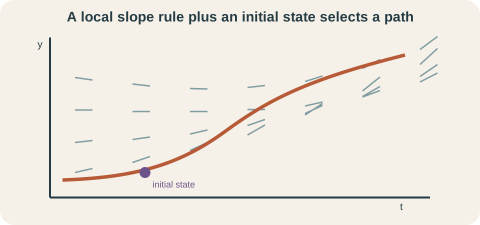
An equation written $y'=f(t,y)$ assigns a slope to each permitted point $(t,y)$. If a solution curve passes through that point, its tangent slope must equal $f(t,y)$. The equation therefore describes local motion through a plane of possible time-state pairs. It does not directly list the entire curve. Integration or another solution method connects those local instructions into a trajectory.

Consider $y'=ky$. The constant $k$ measures proportional rate, and $y$ is the current state. When $k>0$ and $y>0$, the derivative is positive, so solutions increase. Larger values of $y$ produce larger positive slopes. When $k<0$ and $y>0$, the derivative is negative, so solutions decay toward smaller values.

The local-rule viewpoint remains useful when no elementary formula exists. A direction field draws short segments with slope $f(t,y)$ across the plane. A solution curve must stay tangent to those segments. Numerical algorithms follow the same idea by taking finite steps in directions prescribed by the equation. Geometry and computation therefore grow directly from the derivative rule.

Classify order and dimensional state

The order of an ODE is the highest derivative present. The equation $y'+3y=0$ is first order. The equation $y''+4y=0$ is second order because $y''$ is its highest derivative. An equation containing $y'''$ but no higher derivative is third order. Order helps determine how much independent auxiliary information is normally needed.

A higher-order equation contains hidden state components. In mechanics, position $x(t)$ alone does not specify future motion when acceleration depends on the current state. Velocity $v(t)=x'(t)$ must also be known. A second-order equation can therefore be rewritten as two coupled first-order equations by setting $x_1=x$ and $x_2=x'$. This state-space viewpoint connects scalar equations with systems of ODEs.

An $n$th-order equation generally requires $n$ independent initial conditions to select one local trajectory under suitable existence and uniqueness conditions. A second-order motion equation might specify $x(t_0)=x_0$ and $x'(t_0)=v_0$. These conditions provide initial position and velocity. Repeating the same condition twice would not supply two independent pieces of information. Order guides, but does not alone guarantee, a well-posed problem.

Distinguish linear and nonlinear equations

A linear ODE is linear in the unknown function and its derivatives. A general second-order linear equation can be written $a_2(t)y''+a_1(t)y'+a_0(t)y=g(t)$, where the coefficient functions depend only on the independent variable. The unknown $y$ and its derivatives appear only to the first power and are not multiplied together. The function $g(t)$ is an external forcing term. If $g(t)=0$, the equation is homogeneous.

The equation $y'+t^2y=\sin t$ is linear because $y$ and $y'$ appear linearly. The equation $y'=y^2$ is nonlinear because the dependent variable is squared. The equation $y''+yy'=0$ is nonlinear because $y$ multiplies its derivative. Nonlinearity can produce multiple equilibria, finite-time blow-up, bifurcations, and other behavior unavailable in simple linear models. Classification influences which solution methods apply.

Linear does not mean visually straight or easy in every case. It describes algebraic dependence on the unknown function. Coefficients may vary with time, and closed-form solutions may still be difficult. Nonlinear does not mean unsolvable; some nonlinear equations separate or transform exactly. Classification organizes structure rather than assigning a universal difficulty score.

Distinguish autonomous and nonautonomous equations

An autonomous first-order equation has the form $y'=f(y)$ with no explicit independent-variable appearance. Its rate depends only on the current state. The same state value therefore produces the same derivative regardless of time. Population growth with constant parameters often begins with an autonomous model. Equilibria occur at states $y_*$ satisfying $f(y_*)=0$.

A nonautonomous equation has explicit dependence on the independent variable, such as $y'=\cos t-y$. External schedules, seasonal forcing, and time-varying inputs commonly create this form. The same state can have different rates at different times. A phase-line analysis no longer captures the whole rule by state alone. Time must remain part of the complete description.

Any nonautonomous equation can be embedded in a higher-dimensional autonomous system by treating time as a state with $t'=1$. This transformation clarifies why the state must include every quantity needed to determine future rates. It does not remove time dependence from the physical situation. Instead, it expands the state space. Complete-state thinking is one of the central ideas of dynamical systems.

Understand families and initial conditions

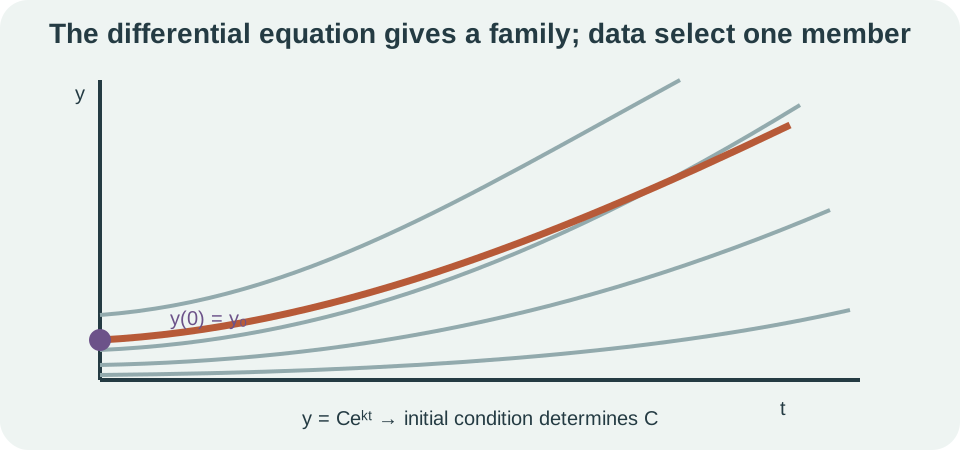
The growth equation $y'=ky$ has the family of solutions $y(t)=Ce^{kt}$, where $C$ is an arbitrary constant. Differentiating gives $y'=Cke^{kt}=ky$, so every value of $C$ produces a solution. The differential equation alone does not select one family member. Each constant corresponds to a different starting value. A first-order solution family generally contains one arbitrary constant.

An initial condition selects a solution at a specified independent-variable value. If $y(0)=y_0$, then substitution into the family gives $y_0=Ce^{k\cdot0}=C$. Therefore the initial-value solution is $y(t)=y_0e^{kt}$. The pair consisting of the equation and initial condition is called an initial-value problem. The initial state anchors the local rate rule to one trajectory.

Units constrain the parameters. If $t$ is measured in seconds, the exponent $kt$ must be dimensionless, so $k$ has units $\frac{1}{\mathrm{second}}$. The constant $y_0$ carries the same unit as $y$. For example, a population model might use individuals for $y$ and inverse years for $k$. Exponential notation does not excuse dimensional inconsistency.

Distinguish initial and boundary conditions

Initial conditions specify all required data at one independent-variable value. For a second-order equation, one might prescribe $y(0)=2$ and $y'(0)=-1$. This describes an initial state containing both position-like and velocity-like information. Evolution problems naturally use such data. Numerical time integration usually begins from the same kind of complete state.

Boundary conditions specify information at more than one independent-variable value. A deflected beam might satisfy $y(0)=0$ and $y(L)=0$ at two supports separated by length $L$. A temperature profile might be fixed at both ends of a rod. Boundary-value problems are not generally solved by simply marching from one endpoint without adjustment. Only selected trajectories may satisfy both boundaries.

The same differential equation can behave differently under initial and boundary conditions. Initial-value uniqueness does not automatically guarantee that a boundary-value problem has one solution. A boundary problem can have no solution, one solution, or many solutions. The type and placement of auxiliary data matter. “Solving the ODE” must include satisfying the actual conditions supplied.

Use analytic, qualitative, and numerical viewpoints

An analytic solution is an exact relationship expressed through known functions, implicit equations, series, or integrals. Exact formulas reveal parameter dependence and may support direct differentiation or limiting analysis. They are powerful when available. However, a formula can be difficult to interpret or evaluate. Many important ODEs have no solution expressible with elementary functions.

A qualitative analysis studies signs, equilibria, stability, monotonicity, bounds, and long-term behavior without requiring a complete formula. For $y'=f(y)$, a phase line marks equilibrium states and arrow directions. Direction fields reveal how slopes vary across the plane. Conservation laws can restrict trajectories to particular sets. Qualitative conclusions often remain meaningful when parameters are uncertain.

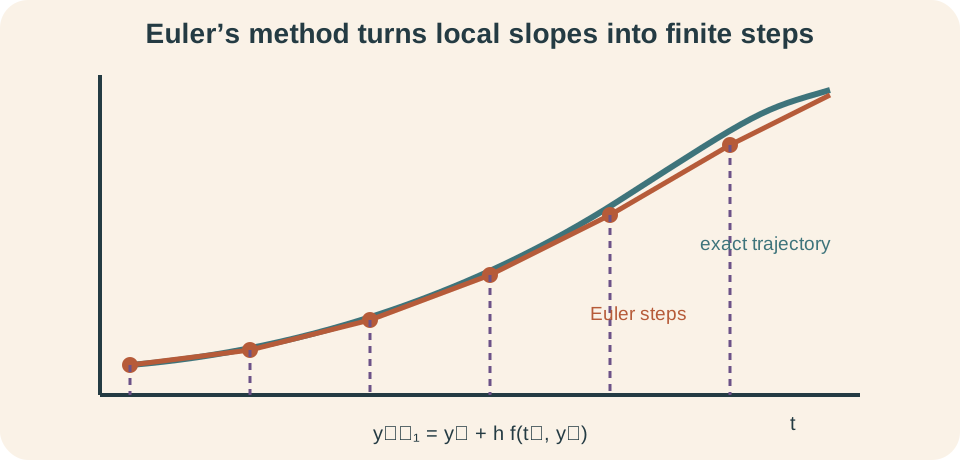
A numerical solution approximates values on a discrete mesh. Euler’s method uses $y_{n+1}=y_n+h f(t_n,y_n)$, where $h$ is the step size. The subscript $n$ indexes an approximate time point, not a derivative. More advanced methods combine several rate evaluations to improve accuracy and stability. Reliable modeling usually compares all three viewpoints rather than treating them as competitors.

Verify a candidate solution completely

To verify a candidate, first confirm that it has the required derivatives on the stated interval. Then substitute the function and derivatives into the differential equation. Simplify both sides until equality is clear. Finally, check every initial or boundary condition. A function satisfying only the equation but not the auxiliary data is not a solution of the full problem.

For $y'=2ty$ with $y(0)=3$, consider $y=3e^{t^2}$. The chain rule gives $y'=3e^{t^2}(2t)=6te^{t^2}$. The right side is $2ty=2t(3e^{t^2})=6te^{t^2}$, so the differential equation holds. The initial value is $y(0)=3e^0=3$. Both requirements are satisfied.

Verification also checks domain. A formula containing $\ln t$ may satisfy an equation only for $t>0$. A square root may restrict state values, and a denominator may exclude points where it vanishes. Simplifying an expression can conceal such restrictions. State the interval on which the candidate genuinely solves the problem.

Translate a conservation balance into an ODE

Many applied ODEs arise from the balance statement “rate of accumulation equals rate in minus rate out plus generation.” Suppose $S(t)$ is salt mass in a well-mixed tank. Salt enters at mass rate $R_{\mathrm{in}}$. If tank volume is constant at $V$ and liquid exits at volumetric rate $q$, the outgoing salt rate is concentration times outflow. The concentration is $\frac{S}{V}$. Each term in the verbal balance becomes a rate with a defined sign.

The balance becomes $S'=R_{\mathrm{in}}-q\frac{S}{V}$. If $S$ is measured in kilograms and $t$ in hours, then $S'$ has units $\frac{\mathrm{kilograms}}{\mathrm{hour}}$. The inflow $R_{\mathrm{in}}$ must have the same unit. The product $(\frac{\mathrm{liters}}{\mathrm{hour}})(\frac{\mathrm{kilograms}}{\mathrm{liter}})$ also gives kilograms per hour. Unit agreement verifies that the terms can be added or subtracted.

The equation depends on modeling assumptions. Perfect mixing makes the outlet concentration equal the tank concentration. Constant volume requires matched liquid inflow and outflow, even if their salt concentrations differ. Constant $q$, $V$, and $R_{\mathrm{in}}$ may hold only during a specified operating period. The ODE is a compact expression of those assumptions, not a context-free truth.

Analyze equilibria and stability

For an autonomous equation $y'=f(y)$, an equilibrium $y_*$ satisfies $f(y_*)=0$. The constant function $y(t)=y_*$ then has derivative zero and solves the equation. Equilibria represent steady states. They organize nearby motion even when most solutions are not constant. Finding them is often the first qualitative step.

Stability asks how nearby trajectories respond to small perturbations. If arrows on both sides point toward an equilibrium, nearby solutions approach it and the equilibrium is stable in the phase-line sense. If arrows point away, it is unstable. If behavior differs by side, it is semistable. Sign analysis of $f(y)$ can reveal these patterns without solving explicitly.

For logistic growth $P'=rP(1-\frac{P}{K})$ with positive $r$ and $K$, equilibria are $P=0$ and $P=K$. Between zero and $K$, both factors are positive and the population increases. Above $K$, the second factor is negative and the population decreases. Thus $K$ is attracting for positive nearby states, while zero is unstable toward positive perturbations. The parameter $K$ carries population units and represents carrying capacity.

Approximate solutions with Euler’s method

Euler’s method replaces the solution curve locally by its tangent line. Starting from $(t_n,y_n)$, compute the slope $f(t_n,y_n)$ and move forward by step $h$. The update $y_{n+1}=y_n+h f(t_n,y_n)$ adds estimated change to the current state. If $t$ is measured in seconds, $h$ has seconds and $f$ has response units per second. Their product has response units, matching $y_n$.

For $y'=0.5y$ with $y(0)=2.0$ and $h=0.10\,\mathrm{seconds}$, the first slope is $0.5\,\frac{1}{\mathrm{second}}(2.0)=1.0\,\frac{\text{response units}}{\mathrm{second}}$. The update is $y_1=2.0+(0.10\,\mathrm{seconds})(1.0\,\frac{\text{response units}}{\mathrm{second}})=2.1$ response units. The method then reevaluates the rate at the new state. Each step accumulates local approximation error. Repeating the calculation constructs a polygonal approximation across the time interval.

Smaller steps usually improve accuracy for a convergent method, but they increase computation and do not cure an inappropriate model. Some equations are stiff, meaning important time scales differ enough that explicit Euler steps must be extremely small for stability. Comparing results after halving the step is a basic convergence check. Numerical output should never be accepted without sensitivity and qualitative verification. Agreement with known equilibria or invariants supplies another valuable check.

Understand existence and uniqueness

For an initial-value problem $y'=f(t,y)$ and $y(t_0)=y_0$, continuity of $f$ near the initial point supports local existence under a standard theorem. Roughly, a solution curve can begin because the slope rule has no immediate break. Existence may still be only local rather than valid for all time. A trajectory can reach a singularity or become unbounded. The theorem’s neighborhood and hypotheses matter.

Local uniqueness is supported when $f$ is locally Lipschitz in $y$. A continuously differentiable $f$ is locally Lipschitz under common conditions. Uniqueness means two different solution curves cannot pass through the same initial point while obeying the same rule. This property justifies treating the vector field as assigning one future to a complete state. It also explains why solution curves of a well-behaved scalar ODE do not cross in the time-state plane.

Continuity alone does not guarantee uniqueness. The equation $y'=\sqrt{|y|}$ with $y(0)=0$ has the zero solution, but the right side is not locally Lipschitz in $y$ at zero. Other solutions can remain at zero for a chosen waiting time and then depart. The same initial condition therefore selects multiple trajectories. A plotted slope field may look harmless while uniqueness fails at a special state.

Respect domains and model validity

A mathematical solution has an interval of existence. The equation $y'=y^2$ with positive initial value produces a solution that becomes unbounded in finite time. The formula’s denominator reveals where it fails. A numerical method stepping past that point does not extend the true classical solution. Global existence must be proved or justified, not assumed from local solvability.

A physical model may fail before its mathematical solution does. Exponential population growth ignores resource limitation at large populations. A linear spring model may fail beyond the elastic range. A constant-coefficient cooling model may neglect phase change or changing ambient conditions. State the parameter range and time interval over which assumptions are credible.

State variables can also have physical constraints. Population, mass, concentration, and absolute temperature may be required to remain nonnegative. A model or numerical scheme that produces negative values deserves investigation. Sometimes the equation guarantees an invariant nonnegative domain, while an overly large numerical step violates it artificially. Mathematical domain, physical domain, and numerical behavior must be distinguished.

Diagnose common misconceptions

Isolating a derivative is not the same as solving an ODE. The expression $y'=f(t,y)$ gives a slope rule, whereas a solution is an entire function agreeing with that rule throughout an interval. Integrating both sides without accounting for dependence on $y$ can be invalid. Solution methods must respect how variables and derivatives appear. Verification exposes many improper manipulations.

An arbitrary constant is not an optional decoration. It represents a family member needed because differentiation loses constant information. Initial or boundary data determine constants when the problem is well posed. Omitting the constant can discard valid solutions. Dividing by a state factor can also lose an equilibrium solution when that factor may equal zero.

Other errors include dropping units, assuming every ODE has an elementary formula, and trusting numerical output without a step-size check. A direction field is not itself a solution. A local existence theorem does not guarantee global behavior. A physical prediction is not valid outside the assumptions merely because the equation continues. Each correction restores one layer of the full problem.

Practice foundational ODE reasoning

For $y''+3y'+2y=0$, identify the independent variable, unknown function, order, and linearity. State how many independent initial conditions are generally needed. Propose suitable initial conditions with symbols and units for a position model. Explain why specifying position twice at the same time is not enough. Distinguish the equation from its solution family.

Verify that $y=4e^{-2t}$ solves $y'=-2y$ and $y(0)=4$. If $t$ is measured in minutes and $y$ in milligrams, state the units of the coefficient negative two. Then identify the equilibrium and predict whether positive solutions grow or decay. Give the long-term limiting behavior. Include every derivative and condition in the check.

Use one Euler step for $y'=y-t$, $y(0)=1.0$, with $h=0.20\,\mathrm{seconds}$ and compatible response units. State the slope at the initial point and the estimated value at $t=0.20\,\mathrm{seconds}$. Explain what reducing $h$ tests. Identify one reason numerical accuracy would not guarantee model validity. Keep the update dimensionally consistent.

Solutions and reasoning

The unknown is a function $y(t)$ of one independent variable $t$. The equation is second order because $y''$ is the highest derivative, and it is linear and homogeneous. Two independent initial conditions are generally required, such as $y(0)=y_0\,\mathrm{meters}$ and $y'(0)=v_0\,\frac{\mathrm{meters}}{\mathrm{second}}$. Position and velocity specify different state components. Repeating the same position condition adds no new information.

Differentiation gives $y'=-8e^{-2t}$, while $-2y=-8e^{-2t}$, so the equation holds. The initial value is $y(0)=4$. If time is measured in minutes, the coefficient has units $\frac{1}{\mathrm{minute}}$. The equilibrium is $y=0$. Every positive solution decays exponentially toward zero as time increases.

At $(t_0,y_0)=(0,1.0)$, the slope is $f(0,1.0)=1.0$ response unit per second. Euler’s update gives $y_1=1.0+(0.20\,\mathrm{seconds})(1.0\,\frac{\text{response units}}{\mathrm{second}})=1.20$ response units. Halving $h$ tests numerical convergence and step sensitivity. Even a converged calculation can represent a poor physical model. Accuracy of integration and validity of assumptions are separate questions.

Carry the ODE viewpoint forward

An ODE combines a local rule for change with enough auxiliary information to select a trajectory. Order identifies hidden state dimensions and expected data requirements. Linearity and autonomy reveal useful structure. Units connect abstract derivatives with measurable rates. Existence and uniqueness determine whether the mathematical question is well posed.

First-order methods will develop separation, integrating factors, phase lines, and numerical approximation in greater detail. Second-order equations will connect acceleration, oscillation, damping, and forcing. Systems will treat several interacting state variables simultaneously. Each branch extends the same state-and-rate viewpoint. The foundational questions remain unchanged.

When meeting a new ODE, do not begin by searching blindly for a formula. Define the state, independent variable, units, domain, parameters, and auxiliary conditions. Classify the equation and study its qualitative behavior. Solve or approximate it with a method justified by that structure, then verify and interpret the result. That workflow turns differential equations into understandable models of evolving systems.