Integrating Factors Solve Linear First-Order ODEs

A first-order linear differential equation can be written in standard form $y'+p(t)y=q(t)$. The unknown function is $y(t)$, the prime means differentiation with respect to $t$, and the known functions $p(t)$ and $q(t)$ describe the equation’s coefficients and input. The equation is linear because $y$ and $y'$ appear only to the first power and are not multiplied together. Its coefficients may vary with time without destroying linearity. The integrating-factor method solves this entire class on intervals where the coefficients behave appropriately.

The method can look like a mysterious instruction to multiply by an exponential. It becomes understandable when designed backward from the product rule. Multiplication by a carefully chosen function turns the two terms containing $y$ into one exact derivative. Integration then reverses that derivative. The procedure is therefore constructed algebra rather than a memorized trick.

This article derives the factor, explains each symbol, and develops a reliable workflow. It treats constant and variable coefficients, initial conditions, interval restrictions, and physical units. Worked examples include verification in the original equation. Interpretations connect the solution to transient response, accumulated forcing, and linear systems. Common mistakes are repaired by returning to the product-rule identity.

Recognize the linear first-order structure

The general form $a(t)y'+b(t)y=g(t)$ is linear in the unknown function. The coefficient $a(t)$ multiplies the derivative, $b(t)$ multiplies the function, and $g(t)$ is a prescribed input. Standard form requires the coefficient of $y'$ to be one. Divide by $a(t)$ wherever $a(t)\ne0$. This produces $p(t)=\frac{b(t)}{a(t)}$ and $q(t)=\frac{g(t)}{a(t)}$.

Linearity concerns dependence on $y$, not whether the independent variable appears nonlinearly. The equation $y'+t^2y=\sin t$ is linear because $t^2$ and $\sin t$ are known functions of $t$. The equation $y'+y^2=t$ is nonlinear because the unknown is squared. The equation $yy'=t$ is nonlinear because the unknown multiplies its derivative. Classification determines whether this method applies.

The interval of work matters. Dividing by $a(t)$ may exclude points where it vanishes. A coefficient such as $\frac{1}{t}$ is continuous separately on $t>0$ and $t<0$ but not across zero. An initial condition selects the relevant interval. A formula valid on one interval should not be carried through a singular point without new analysis.

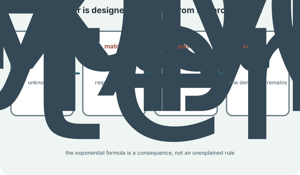
Design the method from the product rule

Begin with $y'+p(t)y=q(t)$ and multiply by an unknown nonzero function $\mu(t)$. The result is $\mu y'+\mu p y=\mu q$. We want the left side to equal the derivative of the product $\mu y$. The product rule gives $(\mu y)'=\mu y'+\mu' y$. Matching the coefficients of $y$ requires $\mu'=\mu p$.

The auxiliary equation $\mu'=p\mu$ is separable. Dividing by nonzero $\mu$ gives $\frac{\mu'}{\mu}=p(t)$. Integrating gives $\ln|\mu|=\int p(t)\,dt+C_0$. Exponentiation gives $\mu=C e^{\int p(t)\,dt}$. Any nonzero constant $C$ can be omitted because it multiplies every later term and cancels.

Choose the simple representative $\mu(t)=e^{\int p(t)\,dt}$. Differentiating it gives $\mu'=p\mu$ by the chain rule. Therefore $\mu y'+\mu p y=\mu y'+\mu' y=(\mu y)'$. The integrating factor works because its logarithmic derivative equals $p$. This identity is the core of the method.

Execute the general solution

After multiplying by $\mu$, the equation becomes $(\mu y)'=\mu q$. Integrate both sides with respect to $t$. This gives $\mu(t)y(t)=\int \mu(t)q(t)\,dt+C$. The constant $C$ represents the one free parameter expected for a first-order equation. Divide by $\mu(t)$ to isolate the unknown.

The general formula is $y(t)=\frac{1}{\mu(t)}\left[\int \mu(t)q(t)\,dt+C\right]$. The brackets group the antiderivative and constant before multiplication by the reciprocal factor. An indefinite integral is acceptable when it can be evaluated clearly. A definite-integral form often handles initial conditions more transparently. Both describe the same solution family.

Do not substitute the formula before the equation is in standard form. If the derivative coefficient is not one, the wrong $p(t)$ produces the wrong factor. After normalization, label $p$ and $q$ explicitly. Differentiate $\mu$ to check $\mu'=p\mu$. This one-line test catches many errors.

Use a definite integral for initial-value problems

Suppose $y(t_0)=y_0$. Integrate $(\mu y)'=\mu q$ from $t_0$ to $t$. The Fundamental Theorem of Calculus gives $\mu(t)y(t)-\mu(t_0)y_0=\int_{t_0}^{t}\mu(s)q(s)\,ds$. The variable $s$ is a dummy integration variable. It prevents confusion between the upper limit $t$ and the quantity being integrated.

Now isolate $y(t)$ by dividing the entire equality by $\mu(t)$. The factor is nonzero because an exponential never vanishes. Keep the initial term and accumulated-input term grouped in the numerator. Use $s$ only inside the integral. This arrangement keeps the initial state visibly separate from later forcing. The resulting expression appears below.

$$y(t)=\frac{\mu(t_0)y_0+\int_{t_0}^{t}\mu(s)q(s)\,ds}{\mu(t)}.$$

The numerator contains the transported initial contribution and accumulated input. The denominator applies the coefficient-driven scaling. Every symbol has a defined role. The first term preserves information supplied at $t_0$. The integral records forcing received between $t_0$ and $t$.

This form satisfies the initial condition automatically. Setting $t=t_0$ makes the integral zero and leaves $y(t_0)=y_0$. It also avoids solving separately for $C$. For theoretical work, the formula exposes how the solution depends on its initial state and forcing. It is the scalar version of variation-of-constants reasoning.

Worked example with constant coefficients

Solve $y'+2y=6$ with $y(0)=1$. Standard form is already present, so $p(t)=2$ and $q(t)=6$. The integrating factor is $\mu=e^{\int2\,dt}=e^{2t}$. Multiplication gives $e^{2t}y'+2e^{2t}y=6e^{2t}$. The left side is $(e^{2t}y)'$.

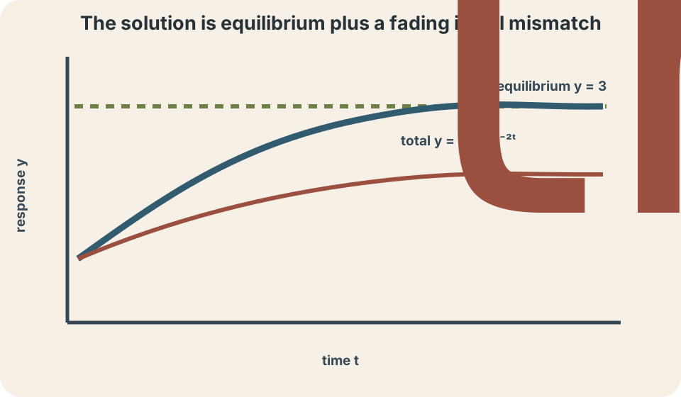
Integrate to obtain $e^{2t}y=3e^{2t}+C$. Dividing by $e^{2t}$ gives $y=3+Ce^{-2t}$. Apply the initial condition: $1=3+C$, so $C=-2$. The solution is $y(t)=3-2e^{-2t}$. It begins at one and approaches three.

Verification should use the original differential equation. Differentiate to get $y'=4e^{-2t}$. Then $y'+2y=4e^{-2t}+2(3-2e^{-2t})=6$. The initial value is $y(0)=3-2=1$. Both the equation and condition are satisfied.

Interpret steady and transient pieces

The constant term three is an equilibrium response. If $y=3$ and $y'=0$, then the equation gives $0+2(3)=6$. The exponential term is a transient. It records how the initial value differs from equilibrium. Its magnitude decays because the exponent is negative.

Writing $y(t)=y_{\mathrm{eq}}+(y_0-y_{\mathrm{eq}})e^{-2t}$ makes the structure explicit. Here $y_{\mathrm{eq}}=3$ and $y_0-y_{\mathrm{eq}}=-2$. The coefficient of the exponential is the initial mismatch. The decay rate $2$ has units reciprocal to those of $t$. A dimensionless exponent requires the product $2t$ to have no unit.

If the coefficient of $y$ were negative, the homogeneous factor could grow rather than decay. The algebraic method would still work. Stability is a separate interpretation based on the sign and accumulated effect of $p(t)$. Integrating factors solve equations whether their solutions decay or grow. Physical plausibility must be assessed from the model.

Variable coefficients require interval awareness

Consider $ty'+2y=t^3$ on $t>0$. Divide by $t$ to obtain $y'+\frac{2}{t}y=t^2$. Now $p(t)=\frac{2}{t}$ and $q(t)=t^2$. The integrating factor is $\mu=e^{\int\frac{2}{t}\,dt}=e^{2\ln t}=t^2$. The restriction $t>0$ justifies writing $\ln t$.

Multiplication gives $t^2y'+2ty=t^4$. The left side is $(t^2y)'$. Integrating gives $t^2y=\frac{t^5}{5}+C$. Therefore $y=\frac{t^3}{5}+\frac{C}{t^2}$. The solution is valid on an interval not crossing zero.

On $t<0$, $\int\frac{2}{t}\,dt=2\ln|t|$, and exponentiation again produces a constant multiple of $t^2$. The same algebraic expression can hold on each side. The constants need not be the same because the intervals are disconnected. No initial value can propagate uniquely through the singular point by this theorem. Domain statements are part of the solution.

Worked example with a nonconstant factor

Solve $y'-\frac{1}{t}y=t^2$ for $t>0$. Here $p(t)=-\frac{1}{t}$ and $q(t)=t^2$. The integrating factor is $\mu=e^{-\ln t}=\frac{1}{t}$. Multiplying produces $\frac{1}{t}y'-\frac{1}{t^2}y=t$. The left side is $\left(\frac{y}{t}\right)'$.

Integrate to get $\frac{y}{t}=\frac{t^2}{2}+C$. Multiplying by $t$ gives $y=\frac{t^3}{2}+Ct$. Notice that the homogeneous term is $Ct$. Substituting it into $y'-\frac{1}{t}y=0$ confirms the homogeneous behavior. The particular term responds to the input $t^2$.

Differentiate the full solution to obtain $y'=\frac{3t^2}{2}+C$. Substitute both $y$ and $y'$ into the normalized equation. Keep the factor $\frac{1}{t}$ outside parentheses until every term is visible. The constant terms should cancel because they form the homogeneous solution. This cancellation is a diagnostic expectation rather than an accidental simplification. The substitution is shown below.

$$y'-\frac{1}{t}y =\frac{3t^2}{2}+C-\frac{1}{t}\left(\frac{t^3}{2}+Ct\right) =t^2.$$

The constant cancels as required. The remaining terms combine to $t^2$. That equals the original right side. Verification therefore confirms the differential equation. It also confirms that the interval-dependent algebra is coherent.

Units constrain coefficient and factor

Suppose $t$ has unit seconds and $y$ has unit concentration $\mathrm{\frac{mol}{L}}$. Then $y'$ has unit $\mathrm{\frac{mol}{L\,s}}$. In $y'+p(t)y=q(t)$, the product $py$ must have the same unit. Therefore $p$ must have unit $\mathrm{\frac{1}{s}}$. The input $q$ must have concentration per time.

The exponent $\int p(t)\,dt$ must be dimensionless. Multiplying $\mathrm{\frac{1}{s}}$ by $\mathrm s$ cancels units. The integrating factor $\mu$ is then dimensionless under the common formulation. If a derived exponent retains a physical unit, the setup is inconsistent. Dimensional reasoning checks the factor before integration continues.

The constant $C$ inherits the unit of $\mu y$. When $\mu$ is dimensionless, $C$ has the same unit as $y$. In a definite-integral formula, $\mu q\,dt$ also has the unit of $y$. Terms added in the numerator therefore agree. Unit consistency mirrors algebraic consistency.

Mixing models produce linear equations

Let $A(t)$ be solute amount in a well-mixed tank. A standard balance is $\frac{dA}{dt}=\text{rate in}-\text{rate out}$. If volume is constant and outflow concentration is $\frac{A}{V}$, the equation can become $A'+\frac{r}{V}A=r c_{\mathrm{in}}$. The flow rate is $r$, tank volume is $V$, and incoming concentration is $c_{\mathrm{in}}$. The coefficient $\frac{r}{V}$ has unit reciprocal time.

The integrating factor is $\mu=e^{(r/V)t}$ for constant parameters. The solution separates into an equilibrium amount and a decaying initial mismatch. The equilibrium is $A_{\mathrm{eq}}=Vc_{\mathrm{in}}$. This makes physical sense because equilibrium tank concentration matches incoming concentration. Algebra and material balance agree.

The model assumes instantaneous uniform mixing, constant volume, fixed flow, and fixed incoming concentration. Real tanks can have dead zones, delays, or time-varying volume. Changing assumptions changes the equation and perhaps its linearity. A polished solution states the model boundary. Mathematical exactness cannot repair an inappropriate physical model.

RC circuits use the same structure

For a resistor–capacitor circuit, a common voltage equation is $RC\frac{dV_C}{dt}+V_C=V_{\mathrm{in}}(t)$. Divide by $RC$ to reach standard form. This gives $V_C'+\frac{1}{RC}V_C=\frac{1}{RC}V_{\mathrm{in}}(t)$. The product $RC$ has units seconds. Its reciprocal is a rate.

The integrating factor is $\mu=e^{t/(RC)}$ for constant resistance and capacitance. The quantity $\tau=RC$ is the time constant. With constant input, the transient decays as $e^{-t/\tau}$. After one time constant, its magnitude is multiplied by $e^{-1}$. The same mathematics described the earlier approach to equilibrium.

Circuit interpretation must retain sign convention and initial capacitor voltage. A discontinuous input can still be handled piecewise. Capacitor voltage remains continuous in the ideal finite-current model, while its derivative can change at a switching time. Each time interval receives its own forcing expression. Continuity connects the interval solutions.

Relation to homogeneous and particular solutions

The associated homogeneous equation is $y'+py=0$. Its solution is $y_h=C e^{-\int p\,dt}=\frac{C}{\mu}$. This is the free response that carries initial information. The nonhomogeneous equation adds forcing $q$. A particular solution accounts for that input.

The integrating-factor formula displays both pieces. The constant term produces the free response. The integral term produces a response to the input. Their sum uses the superposition property of a linear equation. This separation supports both calculation and interpretation. In symbols, the decomposition is shown below.

$$y=\frac{C}{\mu}+\frac{1}{\mu}\int\mu q\,dt.$$

The first term is homogeneous, and the second is one particular response. Their sum works because the differential operator is linear. Superposition applies to the response. If the input is zero, only the homogeneous contribution remains. If the initial mismatch is zero, the forced contribution can still be nonzero.

Different choices of antiderivative can shift a constant between the two pieces. The complete family remains unchanged. A particular solution is not unique because adding a homogeneous solution creates another one. Initial conditions remove the ambiguity. Decomposition is interpretive even when the total solution is fixed.

Common mistakes and repairs

The most common mistake is reading $p(t)$ before normalizing the derivative coefficient. Divide first. Then rewrite the equation with the $y'$ term, the $y$ term, and the input clearly separated. Circle $p(t)$. Test $\mu'=p\mu$ before using the factor.

Another mistake is multiplying only some terms by $\mu$. Every term on both sides must be multiplied. Write the expanded equation before compressing the left side. Compare it directly with $(\mu y)'=\mu y'+\mu' y$. This prevents a missing factor on $q$.

A third mistake is integrating $\mu y'$ and $\mu p y$ separately without recognizing the product derivative. Their individual antiderivatives may be difficult or unavailable. The method exists precisely to package them. Once $(\mu y)'$ is identified, integrate the whole derivative. Return to the designed identity whenever manipulation becomes unclear.

A reliable solution workflow

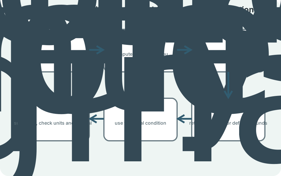
First identify an interval and put the equation in standard form. Confirm that $p(t)$ and $q(t)$ are defined and continuous where the initial value lies. Record units when the equation models a physical system. Distinguish the unknown from prescribed inputs. Classify the equation before choosing the method.

Second compute $\mu=e^{\int p\,dt}$ and verify $\mu'=p\mu$. Multiply every term by $\mu$. Rewrite the left side as $(\mu y)'$. Integrate and isolate $y$. Use a definite integral when an initial value is available.

Third apply conditions and verify the result in the original equation. Check the initial value separately. State the interval of validity. Interpret homogeneous and forced pieces. Examine units, limiting behavior, and equilibrium when applicable.

Retrieval practice and synthesis

Without looking back, derive $\mu=e^{\int p\,dt}$ from the product rule. Begin with an unknown multiplier. Match the coefficient of $y$ rather than quoting the final formula. Explain why a nonzero multiplicative constant in $\mu$ is irrelevant. Then state the interval assumptions required.

Solve $y'+3y=2e^t$ with an unspecified constant. Identify the homogeneous term before evaluating the particular integral. Differentiate the final expression and substitute it into the original equation. Explain which part remembers initial data. State the units that coefficient three must have if $t$ is measured in seconds.

Compare integrating factors with separation of variables. Some equations belong to both classes, but neither class contains the other. Separation rearranges functions of $y$ and $t$ onto opposite sides. Integrating factors exploit linearity and the product rule. Choosing a method begins with structural recognition rather than surface resemblance.