The Fundamental Theorem of Calculus

The Fundamental Theorem of Calculus connects two ideas that initially seem different: local rate and global accumulation. Differentiation examines change at an instant, while integration combines change across an interval. The theorem proves that each process can undo the other under precise hypotheses. Its first part differentiates an accumulation function, and its second part evaluates accumulation with an antiderivative. This lesson develops both directions from meaning, then applies them to moving bounds, net change, units, and interpretation.

Learning objectives and the theorem’s architecture

By the end of this lesson, you will state and justify both parts of the Fundamental Theorem. You will differentiate accumulation functions with fixed, moving, and two-variable bounds. You will evaluate definite integrals using antiderivatives and endpoint subtraction. You will reconstruct quantities from rate data with correct units. You will also distinguish net change from total amount of change.

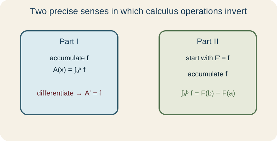
The theorem has two directions because “inverse” can be used in two ways. Begin with a continuous rate $f$, accumulate it, and then differentiate; Part I recovers $f$. Begin with a function $F$, differentiate it to $f$, and then accumulate $f$; Part II recovers the change $F(b)-F(a)$. Neither direction says that symbols simply cancel without conditions. Continuity, interval orientation, and the chain rule determine when each statement applies.

The conceptual map below places accumulation functions between rates and net changes. A fixed lower limit supplies a reference state, while the moving upper limit determines how much has accumulated. An antiderivative provides another function with the same local rate. Comparing those functions proves the endpoint formula. The two parts therefore reinforce one coherent principle rather than two unrelated rules.

Build an accumulation function

Let $f$ be continuous and define $A(x)=\int_a^x f(t)\,dt$. The lower limit $a$ is fixed, while the upper limit $x$ varies. The symbol $t$ is a dummy integration variable that labels positions inside the integral. Using $t$ avoids confusing the running variable with the upper limit. The value $A(x)$ is signed accumulation from $a$ to $x$.

At the reference point, $A(a)=0$ because an interval with identical bounds has zero signed width. If $f$ remains positive, $A$ increases as the upper endpoint moves right. If $f$ is negative, $A$ decreases because new signed area is negative. The graph of $A$ records accumulated balance, not the height of $f$ itself. Its slope will turn out to equal the current height of $f$.

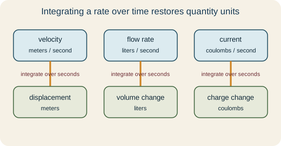
Accumulation has units. If $f(t)$ has units of liters per second and $dt$ contributes seconds, then $A(x)$ has liters. If $f$ is velocity in meters per second, the accumulation is displacement in meters. This unit multiplication anticipates why differentiating $A$ returns rate units. Dimensional reasoning supports the theorem’s interpretation even before its proof.

Prove Part I through local averages

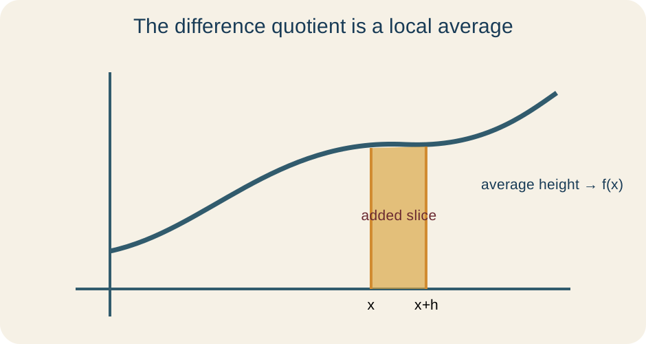
The difference quotient for $A$ is $\frac{A(x+h)-A(x)}{h}$. Additivity of definite integrals makes the numerator $\int_x^{x+h}f(t)\,dt$. Thus the quotient is $\frac{1}{h}\int_x^{x+h}f(t)\,dt$. For positive $h$, this is the average value of $f$ on the short interval from $x$ to $x+h$. The same orientation-aware expression works as $h$ approaches zero from either side.

Continuity forces values of $f(t)$ near $x$ to be close to $f(x)$. Consequently, the average over a shrinking interval is squeezed between nearby minimum and maximum values, both approaching $f(x)$. Taking the limit gives $A'(x)=f(x)$. The prime denotes differentiation with respect to $x$. This statement is Part I of the Fundamental Theorem.

The proof explains more than the formula. A thin additional slice of accumulation has approximate amount $f(x)h$. Dividing that change by the slice width $h$ leaves approximately $f(x)$. As the width shrinks, continuity makes the approximation exact in the limit. The diagram below visualizes the added slice and the average-height argument.

Understand continuity and its limits

Continuity is sufficient for Part I because it controls local averages. If $f$ has a jump at $x$, the accumulation may still be defined, but its derivative there may fail to exist. A right-hand difference quotient can approach the right-hand value while a left-hand quotient approaches the left-hand value. Unequal one-sided limits prevent a derivative. Thus integration can smooth a function without erasing every discontinuity’s effect.

At points where a less regular integrand is continuous, the same local conclusion often remains valid. More advanced versions weaken the hypotheses substantially, but an introductory theorem uses continuity because it is clear and reliable. Do not infer that an integrable function must be continuous. Do not infer that its accumulation function is differentiable at every point. Match the conclusion to the stated theorem.

Endpoints require one-sided interpretation. On a closed interval, an accumulation function may have a right derivative at the left endpoint or a left derivative at the right endpoint. Standard two-sided differentiability is discussed at interior points. Contexts such as time beginning at zero often make a one-sided rate meaningful. State which derivative is intended when the domain has a boundary.

Differentiate moving upper limits

Suppose $G(x)=\int_a^{g(x)}f(t)\,dt$. Define $A(u)=\int_a^u f(t)\,dt$, so $G(x)=A(g(x))$. Part I gives $A'(u)=f(u)$. The chain rule then gives $G'(x)=f(g(x))g'(x)$. The factor $g'(x)$ measures how quickly the moving endpoint changes.

For $G(x)=\int_2^{x^3}\cos t\,dt$, the integrand is evaluated at the upper bound to give $\cos(x^3)$. The upper bound’s derivative is $3x^2$. Therefore $G'(x)=3x^2\cos(x^3)$. Omitting $3x^2$ would ignore the chain rule. Replacing $t$ by $x$ before evaluating the bound would confuse the dummy variable’s role.

If the upper bound moves backward as $x$ increases, then $g'(x)$ is negative. The chain-rule factor automatically reverses the accumulation rate. This is not an extra sign rule but a geometric consequence of endpoint motion. Always identify the outer accumulation function and the inner bound function. Then apply Part I and the chain rule in that order.

Handle lower and two moving bounds

Reversing integral bounds changes sign. Therefore $\int_{g(x)}^a f(t)\,dt=-\int_a^{g(x)}f(t)\,dt$. Differentiation gives $-f(g(x))g'(x)$. The minus sign comes from lower-bound orientation. It is separate from any sign already contained in $g'(x)$.

When both bounds move, insert a fixed reference point $c$. Write $\int_{u(x)}^{v(x)}f(t)\,dt=\int_c^{v(x)}f(t)\,dt-\int_c^{u(x)}f(t)\,dt$. Differentiating gives $f(v(x))v'(x)-f(u(x))u'(x)$. The upper contribution is added and the lower contribution is subtracted. Each bound also receives its own chain-rule derivative.

For $H(x)=\int_{sin x}^{x^2}e^{t^2}\,dt$, the upper contribution is $2xe^{x^4}$. The lower contribution is $e^{sin^2x}\cos x$ and must be subtracted. Thus $H'(x)=2xe^{x^4}-e^{sin^2x}\cos x$. No elementary antiderivative of $e^{t^2}$ is needed. Part I differentiates the accumulation directly.

Prove Part II with equal derivatives

Let $F'(x)=f(x)$ on $[a,b]$, and define $A(x)=\int_a^x f(t)\,dt$. Part I gives $A'(x)=f(x)$. Therefore $A'$ and $F'$ are equal. Two functions with equal derivatives on an interval differ by a constant. Hence $A(x)=F(x)+C$ for some constant $C$.

Evaluate at $x=a$. Since $A(a)=0$, the equation becomes $0=F(a)+C$, so $C=-F(a)$. Therefore $A(x)=F(x)-F(a)$. Setting $x=b$ gives $\int_a^b f(x)\,dx=F(b)-F(a)$. This is Part II of the Fundamental Theorem.

The result converts a limiting sum into endpoint evaluation. It does not redefine the definite integral; rather, it proves a powerful method for computing it. Any antiderivative of $f$ may be used because added constants cancel. The notation $[F(x)]_a^b$ abbreviates $F(b)-F(a)$. Read it as upper endpoint value minus lower endpoint value.

Evaluate definite integrals carefully

Evaluate $\int_1^3(2x+4)\,dx$. One antiderivative is $F(x)=x^2+4x$. Part II gives $[x^2+4x]_1^3$. Substitution produces $(9+12)-(1+4)=16$. Parentheses protect the subtraction of the entire lower-endpoint value.

No $+C$ appears in the final definite-integral value. If one writes $F(x)+C$, endpoint subtraction gives $(F(b)+C)-(F(a)+C)=F(b)-F(a)$. The constants cancel. Adding an arbitrary constant to the numerical result would incorrectly turn one accumulation into a family. Indefinite and definite integrals answer different kinds of questions.

Check the sign against the graph. If the integrand is positive throughout an interval with $a<b$, the definite integral should be positive. Reversing the bounds should negate the result. Splitting at a point should preserve additivity. These qualitative checks catch endpoint-order and arithmetic errors.

Apply the net-change theorem

If $Q'(t)$ is the rate of change of $Q$, Part II gives $Q(b)-Q(a)=\int_a^bQ'(t)\,dt$. Rearranging yields $Q(b)=Q(a)+\int_a^bQ'(t)\,dt$. Final amount equals initial amount plus accumulated rate. This is the net-change theorem. It is the Fundamental Theorem stated in application language.

Suppose water enters a tank at $r(t)=\left(2.0\,\frac{\mathrm{L}}{\mathrm{s}^2}\right)t+1.0\,\frac{\mathrm{L}}{\mathrm{s}}$ for $0\le t\le4.0\,\mathrm{s}$. An antiderivative is $\left(1.0\,\frac{\mathrm{L}}{\mathrm{s}^2}\right)t^2+\left(1.0\,\frac{\mathrm{L}}{\mathrm{s}}\right)t$. Endpoint subtraction gives $20\,\mathrm{L}$. Rate multiplied by time contributes volume units. Add the initial tank volume only if the final volume, rather than volume added, is requested.

Electrical current gives another unit-explicit example. Current has units $\frac{\mathrm{C}}{\mathrm{s}}$, meaning coulombs of charge per second. If $I(t)=2.0\,\frac{\mathrm{C}}{\mathrm{s}}$ for $5.0\,\mathrm{s}$, accumulated charge is $\int_0^{5.0\,\mathrm{s}}I(t)\,dt=10\,\mathrm{C}$. A negative current would contribute negative net charge under the chosen sign convention. Units and sign conventions must be stated together.

Distinguish net change from total variation

The definite integral of a rate gives net change, so positive and negative contributions can cancel. If velocity is positive for part of a trip and negative later, integrating velocity gives displacement. Displacement compares final position with initial position. It can be zero even after substantial motion. Cancellation is appropriate because direction matters.

Total distance traveled is instead $\int_a^b|v(t)|\,dt$. The absolute value makes every contribution nonnegative. Similarly, integrating $|Q'(t)|$ measures total variation in a differentiable quantity. Total variation counts all movement rather than only the final balance. Net change and total variation answer different questions.

To compute total variation, find where the rate changes sign and split the interval there. On each subinterval, interpret the sign or integrate the absolute value correctly. A graph of the rate helps identify those transitions. Do not apply absolute value automatically when the context asks for net balance. Translate the requested quantity before selecting the integrand.

Use a reliable decision process

When differentiating an integral, first identify which bounds depend on the differentiation variable. Evaluate the integrand at each moving bound. Multiply by that bound’s derivative. Add upper-bound contributions and subtract lower-bound contributions. An elementary antiderivative is not required for this process.

When evaluating a definite integral, find one function whose derivative is the integrand. Substitute the upper endpoint and subtract the entire lower-endpoint value. Do not include an arbitrary constant in the final number. Check sign, approximate size, and units. If no elementary antiderivative exists, Part II may not supply a simple closed-form computation.

When reconstructing a quantity from a rate, retain the initial value explicitly. Decide whether the integral represents net change, total amount, or another signed balance. Label variables and units before calculating. State assumptions about continuity and the time interval. Interpret the endpoint result in a complete sentence.

Guided practice and synthesis

Differentiate $J(x)=\int_1^{\sqrt{x}}\ln(1+t^2)\,dt$ for $x>0$. Evaluate the integrand at $\sqrt{x}$ to get $\ln(1+x)$. The derivative of $\sqrt{x}$ is $\frac{1}{2\sqrt{x}}$. Therefore $J'(x)=\frac{\ln(1+x)}{2\sqrt{x}}$. The domain condition supports the square root and its derivative.

Evaluate $\int_0^2(3x^2-1)\,dx$. An antiderivative is $x^3-x$. Endpoint subtraction gives $(8-2)-(0-0)=6$. The positive result is consistent with the larger positive area on the interval. No arbitrary constant remains.

For independent synthesis, let $R(t)$ be a signed material-flow rate in kilograms per hour. Write a formula for the amount at $6.0\,\mathrm{h}$ in terms of the initial amount and $R$. Then explain how to compute total material moved if reverse flow is physically counted as positive throughput. State the units of each integral. Finally, describe the continuity assumption needed to apply the elementary version of the theorem directly.

Connection forward

The Fundamental Theorem proves that continuous local rates and global accumulation determine one another. Part I differentiates accumulation, while Part II evaluates accumulation through an antiderivative. The chain rule handles moving bounds, and orientation supplies lower-bound signs. Net-change applications translate these results into physical and scientific language. Units and qualitative checks keep the symbols connected to meaning.

The most durable approach is to decide which direction of the theorem the problem needs. A derivative outside an integral usually signals Part I. Fixed numerical bounds and an available antiderivative usually signal Part II. A known initial amount and a rate signal net change. A question about all movement rather than final balance may require an absolute value.

Techniques of integration expand the collection of antiderivatives available for Part II. Differential equations use rates and initial values to reconstruct unknown functions. Numerical integration approximates definite integrals when antiderivatives are unavailable. Accumulation functions also appear throughout probability and applied modeling. The theorem remains the bridge that explains why local and global descriptions fit together.