The Definite Integral

A definite integral accumulates many small signed contributions across an interval. It is defined by a limit of finite sums, not by the antiderivative shortcut learned later. Rectangle widths shrink while the number of contributions grows, and a stable limiting total becomes the integral. This definition explains signed area, physical units, numerical approximation, and the distinction between net and total change. The lesson develops those meanings before connecting them to exact evaluation through the Fundamental Theorem.

Learning objectives and the accumulation idea

By the end of this lesson, you will construct and interpret Riemann sums. You will explain the definite integral as a limit independent of sample-point choice. You will use signed area, orientation, additivity, linearity, and comparison properties. You will distinguish net accumulation from total accumulated magnitude. You will also calculate average value and reason about approximation error and units.

Accumulation combines a rate-like or density-like quantity with small input widths. Each product estimates a contribution from one short subinterval. Adding those products produces a finite approximation. Refining the partition makes each local approximation more faithful. A limit turns the improving approximations into a quantity attached to the entire function and interval.

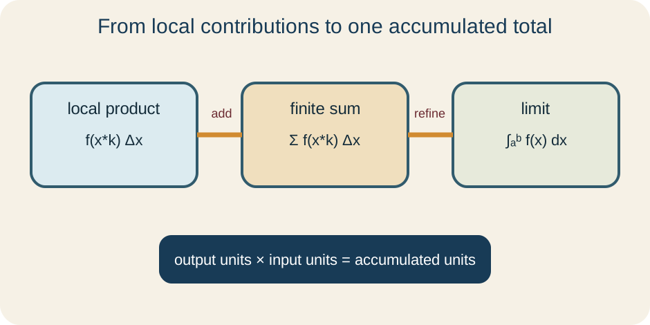
This pattern appears far beyond geometric area. Velocity times a short time interval approximates displacement, flow rate times time approximates volume, and linear density times length approximates mass. The units of the product reveal what is being accumulated. The concept map below connects local contribution, finite sum, and limiting total. It also separates the integral’s definition from later computational methods.

Partition an interval and build a sum

Partition $[a,b]$ into $n$ subintervals. For equal widths, $\Delta x=\frac{b-a}{n}$. The Greek capital delta indicates a change or width, not multiplication by a variable named delta. In the $k$th subinterval, choose a sample point $x_k^*$. The star marks a representative input rather than an exponent.

The Riemann sum is $\sum_{k=1}^{n}f(x_k^*)\Delta x$. The sigma symbol instructs us to add one product for each index $k$ from one through $n$. The function value supplies an approximate height or rate. The factor $\Delta x$ supplies width. Omitting the width leaves a sum with the wrong scale and usually the wrong units.

For unequal partitions, write widths as $\Delta x_k=x_k-x_{k-1}$. The sum becomes $\sum f(x_k^*)\Delta x_k$. Refinement means the largest width approaches zero, not merely that the number of pieces increases. This general version explains why the definition is not tied to equal rectangles. Equal subdivisions are convenient for calculation but not essential to the idea.

Define the definite integral by a limit

If all legitimate Riemann sums approach one finite number as the partition mesh approaches zero, that number is $\int_a^bf(x)\,dx$. The symbol $a$ is the lower limit, $b$ is the upper limit, and $f(x)$ is the integrand. The differential $dx$ identifies the input variable whose widths are accumulating. The integral sign is an elongated S that recalls summation. The result is one number for the specified function and oriented interval.

For equal subdivisions, one may write $\int_a^bf(x)\,dx=\lim_{n\to\infty}\sum_{k=1}^{n}f(x_k^*)\Delta x$. The infinity symbol describes unbounded growth of $n$ rather than a number substituted into the sum. Every sum before the limit is finite. The integral exists when refinement forces the approximations together. A finite rectangle sum is generally not the exact integral.

Continuous functions on closed intervals are Riemann integrable. Continuity is sufficient but not necessary. A bounded function with finitely many jump discontinuities can still be integrable because narrow neighborhoods of the jumps contribute arbitrarily little. Unbounded behavior requires a separate improper-integral definition. Always match a theorem’s conclusion to its stated hypotheses.

Compare left, right, and midpoint sums

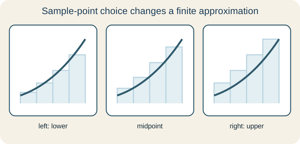
A left sum chooses each subinterval’s left endpoint, while a right sum chooses its right endpoint. A midpoint sum chooses the center. These rules usually give different finite approximations. For an increasing function, left rectangles lie below the graph and right rectangles lie above it. Consequently, left and right sums provide lower and upper estimates when the function is also nonnegative.

The midpoint rule often improves accuracy because overestimates and underestimates within each subinterval partially balance. The trapezoidal rule uses the average of endpoint heights and connects them with line segments. Neither method is automatically exact. Exactness depends on function structure and the chosen rule. Refinement generally improves approximation, but the rate of improvement varies.

Suppose $f(x)=x^2$ on $[0,2]$ and use four equal subintervals. The width is $\Delta x=\frac{2-0}{4}=0.5$. A right sum samples $0.5$, $1.0$, $1.5$, and $2.0$. It is $0.5[(0.5)^2+(1.0)^2+(1.5)^2+(2.0)^2]$. The units are function-output units multiplied by $x$-units.

Interpret signed area and orientation

When $f(x)>0$, a contribution $f(x_k^*)\Delta x$ is positive for left-to-right orientation. When $f(x)<0$, the contribution is negative. Therefore the definite integral measures signed area relative to the horizontal axis. Regions below the axis subtract from regions above it. Signed area is an algebraic balance, not always geometric area.

Reversing bounds changes orientation. By definition and consistent algebra, $\int_b^af(x)\,dx=-\int_a^bf(x)\,dx$. An interval of zero oriented width gives $\int_a^af(x)\,dx=0$. These properties are not cosmetic sign conventions. They allow interval pieces to combine consistently regardless of direction.

Geometric area is nonnegative. To find it, locate where $f$ changes sign and integrate $|f(x)|$, or split the interval and reverse negative contributions. If positive and negative regions have equal magnitude, the definite integral can be zero while geometric area is substantial. State which quantity the problem requests. A picture should show sign as well as shape.

Use additivity, linearity, and comparison

Additivity over intervals states $\int_a^bf=\int_a^cf+\int_c^bf$. The point $c$ may lie between $a$ and $b$, and orientation handles other arrangements. This property mirrors splitting a finite sum into groups. It is useful when formulas or signs change at known points. It also lets measured accumulation over separate periods combine into a total.

Linearity states $\int_a^b(\alpha f+\beta g)=\alpha\int_a^bf+\beta\int_a^bg$ for constants $\alpha$ and $\beta$. Scaling every local contribution scales the accumulated total. Adding integrands adds their local contributions before or after accumulation. Linearity supports unit conversion and superposition. It does not permit nonlinear operations such as moving a square outside an integral.

If $f(x)\le g(x)$ throughout $[a,b]$ with $a<b$, then $\int_a^bf\le\int_a^bg$. More generally, if $m\le f(x)\le M$, then $m(b-a)\le\int_a^bf(x)\,dx\le M(b-a)$. These inequalities compare accumulation to bounding rectangles. They provide reasonableness checks even when an exact value is unknown. Reversed bounds require orientation awareness before applying the inequality.

Track units through accumulation

Integral units equal integrand units multiplied by input units. If velocity is measured in meters per second and time in seconds, the integral has meters. If linear density is kilograms per meter and position is meters, the integral has kilograms. The differential identifies the input unit being accumulated. Units should be reported on numerical answers.

A pump’s flow rate might be measured every $2.0\,\mathrm{min}$ as $3.0$, $3.8$, $4.1$, and $4.5\,\frac{\mathrm{L}}{\mathrm{min}}$. A left estimate over the first $6.0\,\mathrm{min}$ uses the first three recorded rates. It is $(2.0\,\mathrm{min})\left(3.0+3.8+4.1\right)\frac{\mathrm{L}}{\mathrm{min}}=21.8\,\mathrm{L}$. Adding rates without multiplying by time would retain rate units and could not represent volume. The width factor is physically essential.

Dimensional consistency can reveal the wrong integrand. Integrating acceleration over time gives velocity change, not displacement. Integrating power over time gives energy because power is energy per time. Integrating a probability density over its variable gives dimensionless probability. Units do not prove the numerical result, but incompatible units prove the setup is wrong.

Distinguish displacement and distance

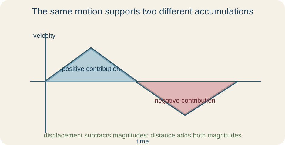
Velocity is a signed rate of position change. Its definite integral over time gives displacement. Positive and negative motion can cancel because displacement compares final position with initial position. Total distance instead accumulates speed $|v(t)|$. The absolute value removes directional sign.

Suppose a cart moves at $4.0\,\frac{\mathrm{m}}{\mathrm{s}}$ for $3.0\,\mathrm{s}$ and then at $-2.0\,\frac{\mathrm{m}}{\mathrm{s}}$ for $2.0\,\mathrm{s}$. Displacement is $(4.0\,\frac{\mathrm{m}}{\mathrm{s}})(3.0\,\mathrm{s})+(-2.0\,\frac{\mathrm{m}}{\mathrm{s}})(2.0\,\mathrm{s})=8.0\,\mathrm{m}$. Distance is $12.0\,\mathrm{m}+4.0\,\mathrm{m}=16.0\,\mathrm{m}$. The negative velocity records direction rather than a negative amount of travel. Both calculations are correct answers to different questions.

For variable velocity, find zeros and sign changes. Split the interval where direction changes. Integrate velocity for displacement and absolute velocity for distance. A velocity-time graph makes each signed region visible. Do not take the absolute value of the final displacement; that loses intermediate travel.

Find average value

The average value of an integrable function on $[a,b]$ is $f_{\mathrm{avg}}=\frac{1}{b-a}\int_a^bf(x)\,dx$. The integral supplies total signed accumulation. Dividing by interval width produces output units again. This mirrors an arithmetic average: total divided by amount of input. The result is one representative height.

Geometrically, the rectangle of height $f_{\mathrm{avg}}$ and width $b-a$ has the same signed area as the function. If $f$ is continuous, the Mean Value Theorem for Integrals guarantees a point $c$ where $f(c)=f_{\mathrm{avg}}$. The theorem does not necessarily identify a unique point. Several inputs may share the same function height. It links an accumulated average to an actual function value.

For $f(x)=2x$ on $[0,3]$, the integral is nine. Dividing by width three gives average value three. This matches the midpoint function value $f(1.5)=3$ because the function is linear. Nonlinear functions need not have average value at the interval midpoint. Use the formula rather than midpoint intuition alone.

Estimate error and judge approximations

Monotonicity provides immediate bounds. If a positive function increases, a left sum underestimates and a right sum overestimates. The difference between them bounds the uncertainty of either estimate relative to the integral. Taking their average gives the trapezoidal estimate for equal subintervals. This bracket is often more informative than one isolated approximation.

Smoothness determines more precise error behavior. Midpoint and trapezoidal errors depend on the second derivative, while Simpson’s rule uses additional curvature information and has higher-order accuracy for smooth functions. Error formulas require stated derivative bounds. Do not quote a numerical tolerance without checking those conditions. More subintervals alone does not explain the size of error.

Graph and units provide independent checks. A positive function bounded above by $M$ on an interval of width $w$ cannot have integral greater than $Mw$. If a rate is approximately constant, the integral should resemble rate times duration. Compare several numerical rules when exact evaluation is unavailable. Consistent values support the estimate but do not replace a theoretical error bound.

Connect definition to the Fundamental Theorem

The definite integral is defined by limiting sums. The Fundamental Theorem later proves that if $F'=f$, then $\int_a^bf(x)\,dx=F(b)-F(a)$. This endpoint formula is an evaluation method, not the original definition. Its power comes from proving that antiderivatives compute the same limit. Keeping definition and theorem distinct clarifies why the shortcut is valid.

An accumulation function $A(x)=\int_a^xf(t)\,dt$ treats the upper bound as variable. Under continuity, the Fundamental Theorem gives $A'(x)=f(x)$. Thus the rate of accumulated area is the current integrand height. This statement connects global sums back to local derivatives. It is the inverse relationship at the heart of calculus.

Numerical integration remains necessary when sampled data are given or an elementary antiderivative is unavailable. The definition supports those methods directly. Exact antiderivatives and numerical sums are not competing meanings. They are different routes to the same accumulated quantity when their hypotheses are satisfied. A responsible solution chooses the route supported by available information.

Guided practice and synthesis

Write a right-endpoint sum for $\int_0^2x^2\,dx$ using $n$ equal pieces. The width is $\Delta x=\frac{2}{n}$. The right endpoint is $x_k=\frac{2k}{n}$. The sum is $\sum_{k=1}^{n}\left(\frac{2k}{n}\right)^2\frac{2}{n}$. Taking the limit as $n\to\infty$ defines the integral.

If $\int_1^4f(x)\,dx=7$ and $\int_4^6f(x)\,dx=-2$, additivity gives $\int_1^6f(x)\,dx=5$. The negative second contribution reduces the net accumulation. It does not mean the second interval has negative geometric area. The sign refers to the integrand relative to the axis. Additional information would be needed to find total area.

For independent synthesis, suppose $2\le f(x)\le5$ on $[1,4]$. Bound the integral using rectangle inequalities and explain the role of interval width. Then describe how reversing the bounds changes the result and the inequalities. Construct a midpoint sum with three equal subintervals in symbolic form. Finally, state what additional information would let you calculate a guaranteed numerical error.

Connection forward

The definite integral is a limit of finite signed sums. Partitions organize local contributions, and refinement makes the total independent of sample choices. Orientation, linearity, additivity, and comparison turn that limit into a flexible mathematical object. Units explain what has accumulated. Absolute values separate total magnitude from net balance.

The strongest solutions keep four layers visible. Define the variable and units, construct the finite approximation, identify the limiting object, and interpret its sign and magnitude. Use graphs and inequalities to check reasonableness. Do not confuse an approximation with an exact result. Do not confuse signed accumulation with geometric area.

The Fundamental Theorem proves that continuous accumulation functions differentiate back to their integrands and that antiderivatives evaluate definite integrals. Numerical methods extend calculation to data and functions without elementary antiderivatives. Probability, physics, economics, and differential equations all use the same accumulation structure. Each discipline gives the local product a different interpretation. The Riemann-sum definition remains the foundation beneath those applications.