Sequences, Series, and Sigma Notation

Sigma notation is a compact instruction for repeated addition. Its index, bounds, and summand jointly determine exactly which terms appear. Careful indexing allows sums to be expanded, compressed, shifted, split, and combined without changing their values. Partial sums then convert an infinite-looking expression into a sequence that can be studied by limits. This lesson develops the notation and transformations that later support Riemann sums and infinite series.

Read the anatomy of a finite sum

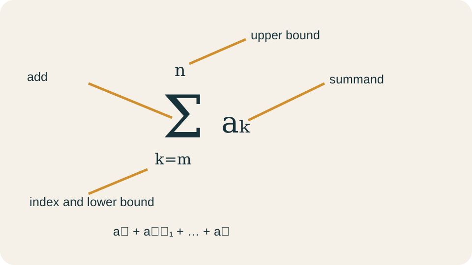
In $\sum_{k=m}^{n}a_k$, the Greek capital sigma, $\sum$, means add. The symbol $k$ is the index of summation. The lower bound $m$ gives the first index value. The upper bound $n$ gives the last index value. The expression $a_k$ is the summand evaluated at each index.

When $m$ and $n$ are integers with $m\leq n$, the expanded sum is $a_m+a_{m+1}+\cdots+a_n$. Both endpoints are included. The number of terms is $n-m+1$. The plus one accounts for inclusive counting. Substituting a small example confirms the formula.

For $\sum_{k=2}^{5}(3k-1)$, the index takes values two, three, four, and five. There are $5-2+1=4$ terms. The summand produces $5,8,11,14$. Their sum is $38$. Every part of the notation contributes information.

Distinguish index from term value

The index tells which substitution to make. It is not automatically equal to the summand. In $\sum_{k=1}^n k^2$, the index values are $1,2,\ldots,n$, while term values are $1^2,2^2,\ldots,n^2$. In $\sum_{k=1}^n a_k$, the sequence rule determines the term values. The index only selects them.

Subscripts and exponents play different roles. The symbol $a_k$ names the $k$th term of a sequence. The symbol $a^k$ raises fixed base $a$ to power $k$. The expression $a_{k^2}$ selects a term at squared index. Careful reading prevents these operations from being interchanged.

Physical indices are commonly dimensionless counts. A summand may still carry units. If $a_k$ is an energy contribution in joules, the sum is measured in joules. The index selects contributions without adding units of its own. A sum can combine only dimensionally compatible terms.

Treat the index as a local variable

The index of summation is a dummy variable whose name is local to the sum. Thus $\sum_{k=1}^nk^2=\sum_{j=1}^nj^2$. The letters differ, but the generated lists agree. Renaming the index does not change the value. Bounds and summand structure must remain aligned.

A variable used outside the sum may be free rather than dummy. In $x\sum_{k=1}^nk$, the symbol $x$ is not controlled by the sigma. It remains an external factor. Renaming $k$ to $x$ would create a collision and obscure scope. Distinct labels keep local and external roles clear.

Nested sums need separate indices. The expression $\sum_{i=1}^m\sum_{j=1}^na_{ij}$ uses $i$ for rows and $j$ for columns. Reusing one index for both levels would be ambiguous. Each sigma controls its own bound variable. Scope rules make complicated summations readable.

Expand a sum systematically

To expand, write the first index, substitute it into the summand, and continue by integer steps through the upper bound. Stop after including the upper endpoint. Parentheses should surround substituted expressions when needed. This procedure is more reliable than guessing a visual pattern. It also exposes the number of terms.

For $\sum_{j=0}^{4}2^j$, substitution gives $2^0+2^1+2^2+2^3+2^4$. The powers are $1,2,4,8,16$. The total is $31$. Five terms appear because $4-0+1=5$. Counting the written terms confirms that both endpoints were included.

For $\sum_{k=-2}^{2}(k^2+1)$, the index list is $-2,-1,0,1,2$. Parentheses matter when squaring negative indices. The values are $5,2,1,2,5$. The total is $15$. Symmetry provides an independent check.

Compress a written pattern

Compression reverses expansion. Identify a term formula, a starting index, an ending index, and an index step. Standard sigma notation assumes consecutive integer steps of one. If the visible pattern skips values, the summand can encode the spacing. Many different sigma forms can represent the same finite list.

The sum $3+5+7+9$ can be written $\sum_{k=1}^{4}(2k+1)$. Substituting one produces three, and substituting four produces nine. It can also be written $\sum_{j=0}^{3}(2j+3)$. The index forms differ but term lists agree. Neither is uniquely privileged.

Before accepting a compressed form, test the first term, last term, and term count. A correct first and last term can still hide the wrong number of intermediate terms. Check the progression rule as well. Compression is an exact encoding task. Three checks make the encoding auditable.

Apply linearity of finite sums

Finite summation distributes over addition. The identity is $\sum_{k=m}^{n}(a_k+b_k)=\sum_{k=m}^{n}a_k+\sum_{k=m}^{n}b_k$. A constant factor can be moved outside, so $\sum_{k=m}^{n}ca_k=c\sum_{k=m}^{n}a_k$. These facts follow by expanding and using ordinary algebra. They are called linearity.

Combining both rules gives $\sum_{k=m}^{n}(ca_k+db_k)=c\sum_{k=m}^{n}a_k+d\sum_{k=m}^{n}b_k$. The constants $c$ and $d$ must not depend on the controlled index $k$. If a factor varies with $k$, it generally cannot be moved outside. The sum of products is not usually the product of sums. Distribution must follow valid algebra.

Evaluate $\sum_{k=2}^{5}(3k-1)$ through linearity. It becomes $3\sum_{k=2}^{5}k-\sum_{k=2}^{5}1$. The index sum is fourteen, and the constant sum has four terms. Therefore the result is $3(14)-4=38$. Expansion and linearity agree.

Sum a constant correctly

If constant $c$ is repeated from $k=m$ through $k=n$, then $\sum_{k=m}^{n}c=c(n-m+1)$. The summand does not contain $k$, but the bounds still control repetition. Forgetting the term count is a common error. The result is not automatically $cn$ unless the lower bound is one. Inclusive counting remains essential.

For $\sum_{k=3}^{7}4$, there are $7-3+1=5$ terms. The sum is $20$. Writing $4(7)$ would incorrectly count seven repetitions. Expanding $4+4+4+4+4$ confirms the answer. Bounds are operational instructions.

If $c$ carries units, multiplication by term count preserves those units. Five payments of $20\,\mathrm{dollars}$ sum to $100\,\mathrm{dollars}$. The count is dimensionless. A rate per time interval may require multiplying each rate by an interval width before summing. Units clarify what the summand represents.

Split and combine sums

A finite sum can be split at an interior index. If $m\leq p<n$, then $\sum_{k=m}^{n}a_k=\sum_{k=m}^{p}a_k+\sum_{k=p+1}^{n}a_k$. The second part begins at $p+1$ to avoid duplicating $a_p$. Every original term appears exactly once. Expanding a short example verifies the partition.

Adjacent sums with the same summand can be combined. The expression $\sum_{k=1}^{5}a_k+\sum_{k=6}^{10}a_k$ equals $\sum_{k=1}^{10}a_k$. If bounds overlap, duplicate terms must be handled. If a gap exists, missing terms cannot be invented. Interval logic applies to index sets.

Splitting is useful when a summand changes formula or when early terms require special treatment. Algorithms also process data in blocks using this principle. Infinite-series proofs often separate a finite prefix from a tail. A finite prefix cannot change convergence of the remaining infinite tail. Index partitions make that reasoning precise.

Shift an index consistently

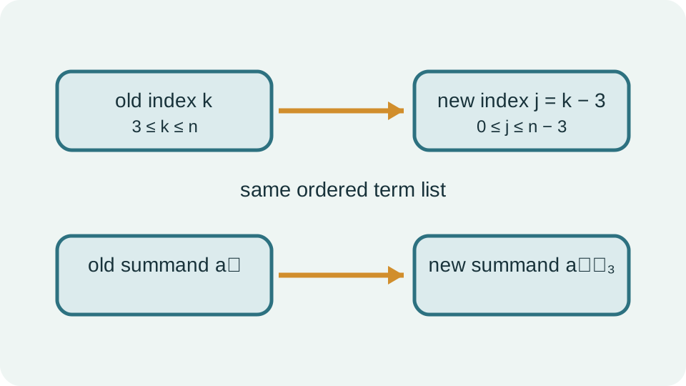
An index shift replaces the dummy variable with a new one. Suppose $j=k-1$. When $k=1$, the new lower index is $j=0$. When $k=n$, the new upper index is $j=n-1$. The summand $a_{k-1}$ becomes $a_j$. Therefore $\sum_{k=1}^{n}a_{k-1}=\sum_{j=0}^{n-1}a_j$.

All three pieces must change consistently: index, bounds, and summand. Changing only the letter is renaming, not shifting. Changing bounds without adjusting the summand changes the term list. The safest method maps the first and last old indices explicitly. Then substitute the inverse relation into the summand.

To rewrite $\sum_{k=3}^{n}a_k$ with an index starting at zero, let $j=k-3$. Then $k=j+3$. The lower bound becomes zero, and the upper bound becomes $n-3$. The equivalent sum is $\sum_{j=0}^{n-3}a_{j+3}$. Expansion confirms the same terms $a_3$ through $a_n$.

Reverse the direction of indexing

Some sums are easier to understand when indices run in reverse order conceptually. Finite addition is commutative, so term order can change without changing the sum. Standard sigma bounds still increase from lower to upper. A substitution such as $j=n-k$ can encode reversal. Bounds and summand must again be transformed.

For $\sum_{k=0}^{n}a_{n-k}$, let $j=n-k$. When $k=0$, $j=n$, and when $k=n$, $j=0$. The listed terms are $a_n,a_{n-1},\ldots,a_0$. Reversing their addition gives $\sum_{j=0}^{n}a_j$. The equality uses both index substitution and commutativity.

Reversal appears in convolution, financial timing, and polynomial coefficients. An early deposit may receive a high growth exponent while a late deposit receives a low exponent. Reindexing can turn backward timing into a standard geometric sum. A timeline should accompany the algebra. It reveals which event belongs to each exponent.

Derive the sum of the first integers

Let $S=1+2+\cdots+n$. Write it again in reverse as $S=n+(n-1)+\cdots+1$. Adding corresponding positions gives $2S=(n+1)+(n+1)+\cdots+(n+1)$. There are $n$ identical pair sums. Therefore $2S=n(n+1)$.

Dividing by two yields $\sum_{k=1}^{n}k=\dfrac{n(n+1)}{2}$. The formula is a polynomial in $n$. It can be verified for small values. For $n=4$, it gives $4(5)/2=10$, matching $1+2+3+4$. Derivation explains the factor one-half.

The identity counts several geometric objects. It gives the number of dots in a triangular arrangement with rows one through $n$. It also counts pairs selected from $n+1$ objects. Multiple interpretations strengthen understanding. The same closed form can arise from algebra, geometry, and counting.

Use standard finite-sum identities

Three common identities are $\sum_{k=1}^{n}1=n$, $\sum_{k=1}^{n}k=\dfrac{n(n+1)}{2}$, and $\sum_{k=1}^{n}k^2=\dfrac{n(n+1)(2n+1)}{6}$. They hold for positive integer $n$. The first counts terms. The second was derived by pairing. The third can be proved by induction or telescoping polynomial identities.

Linearity combines these formulas. For example, $\sum_{k=1}^{20}(2k+3)=2\sum_{k=1}^{20}k+3\sum_{k=1}^{20}1$. Substitution gives $2\left(\dfrac{20(21)}{2}\right)+3(20)=480$. The answer contains twenty terms averaging twenty-four. That average check confirms the total.

Closed forms replace iteration with direct calculation. They are especially useful when $n$ is large or symbolic. A formula should still be checked at $n=1$ and another small index. Such checks cannot prove an identity for every $n$, but they catch transcription mistakes. Proof supplies universality.

Verify identities by induction

Mathematical induction proves statements indexed by positive integers. First verify the base case, often $n=1$. Then assume the formula holds at a general index $n$. This assumption is the induction hypothesis. Finally prove it must then hold at $n+1$.

For the integer-sum formula, assume $\sum_{k=1}^{n}k=\dfrac{n(n+1)}{2}$. Add the next term $n+1$. The new sum is $\dfrac{n(n+1)}{2}+(n+1)=\dfrac{(n+1)(n+2)}{2}$. This matches the claimed formula with $n$ replaced by $n+1$. Base and step complete the proof.

Induction does not explain every formula’s origin. It verifies a proposed pattern once discovered. Pairing explains why the integer-sum form is natural. Algebraic telescoping can reveal other identities. Discovery and proof are distinct mathematical tasks.

Derive a finite geometric sum

Let $S_n=1+r+r^2+\cdots+r^{n-1}$. Multiply by $r$ to obtain $rS_n=r+r^2+\cdots+r^n$. Subtract the shifted sum from the original. Interior powers cancel. The result is $(1-r)S_n=1-r^n$.

For $r\neq1$, divide to obtain $\sum_{k=1}^{n}r^{k-1}=\dfrac{1-r^n}{1-r}$. If $r=1$, the sum contains $n$ copies of one and equals $n$. The excluded value must be handled separately. A zero denominator signals a missing case rather than an infinite result automatically. This case distinction completes the formula without assigning meaning to division by zero.

More generally, $\sum_{k=0}^{n}ar^k=a\dfrac{1-r^{n+1}}{1-r}$ for $r\neq1$. The highest exponent is $n$, so there are $n+1$ terms. That term count explains the exponent $n+1$ in the numerator. Checking $n=0$ reproduces the single term $a$. Indexing controls the closed form.

Define partial sums

For a sequence $(a_k)$, define its partial-sum sequence by $S_n=\sum_{k=1}^{n}a_k$. Each $S_n$ is finite. The sequence $S_1,S_2,S_3,\ldots$ records accumulating totals. It is not the same as the original sequence. Capital notation helps distinguish the two.

Successive partial sums satisfy $S_n-S_{n-1}=a_n$. The newest term is the increment in the total. This discrete difference is analogous to how a derivative describes local change in an accumulated function. Conversely, summing the increments reconstructs the total. Calculus later makes this relationship continuous.

For $a_k=2k+1$, the partial sum is $S_n=\sum_{k=1}^{n}(2k+1)$. Linearity gives $S_n=n(n+1)+n=n^2+2n$. The single term $a_n$ grows linearly, while the accumulated total grows quadratically. Accumulation changes growth order. Evaluating a small value such as $n=2$ checks that both descriptions give the same total.

Define an infinite series with partial sums

The expression $\sum_{k=1}^{\infty}a_k$ is defined through the limit of partial sums. If $\lim_{n\to\infty}S_n=S$ for finite $S$, the series converges to $S$. If no finite limit exists, the series diverges. The infinity symbol is not an upper index that can be reached. It signals a limiting process.

Term convergence to zero is necessary for series convergence. Since $a_n=S_n-S_{n-1}$, convergent partial sums must have increments approaching zero. The converse fails. The harmonic terms $1/n$ approach zero while their partial sums grow without bound. A term test can establish divergence when the term limit is nonzero, but not convergence when it is zero.

Finite index manipulations prepare this analysis. Shifts, splits, and linearity can reorganize partial sums. For infinite series, such operations require convergence care beyond purely finite algebra. Rearranging conditionally convergent series can change values. Precalculus builds the notation that calculus later qualifies.

Connect sigma notation to Riemann sums

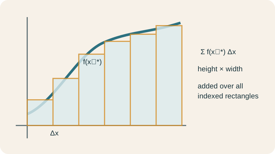
A Riemann sum approximates area or accumulated change by adding many rectangular contributions. A typical form is $\sum_{k=1}^{n}f(x_k^*)\Delta x$. The sample point $x_k^*$ selects a function height. The width $\Delta x$ supplies horizontal units. Their product has units of accumulated quantity.

For interval $[a,b]$ divided into $n$ equal pieces, $\Delta x=\dfrac{b-a}{n}$. A right-endpoint choice uses $x_k=a+k\Delta x$. The index identifies each subinterval. The sigma then adds all rectangular contributions. Bounds guarantee that exactly $n$ pieces appear.

The definite integral is a limit of such sums as the maximum subinterval width approaches zero. Accurate index notation prevents missing or duplicating rectangles. Units reveal whether a sum represents area, distance, mass, or another accumulation. Finite sigma skills become foundational calculus language. The transition is structural rather than cosmetic.

Model discrete accumulation

Suppose monthly contribution $c_k$ varies with month $k$. Total contributed through month $n$ is $C_n=\sum_{k=1}^{n}c_k$. If interest is absent, this is direct accumulation. If each contribution grows for a different number of months, the summand includes a timing factor. Indexing expresses the financial schedule.

For end-of-month deposits of fixed amount $D$ with monthly growth factor $r$, the balance after deposit $n$ is $B_n=\sum_{k=1}^{n}Dr^{n-k}$. The first deposit receives exponent $n-1$, and the last receives exponent zero. Letting $j=n-k$ reindexes the sum as $D\sum_{j=0}^{n-1}r^j$. The standard geometric formula now applies. The reindexed expression preserves every deposit while listing the growth periods in ascending order.

Units remain dollars because $D$ is in dollars and $r$ is dimensionless. The index and exponent encode timing rather than physical units. A timeline verifies which deposit grows longest. Reindexing simplifies the algebra without altering the financial events. This is the practical purpose of a valid index shift.

Diagnose common sigma errors

One error is forgetting the plus one in inclusive term count. Another is changing bounds without changing the summand during an index shift. Expanding the first and last terms on both sides exposes these errors. A valid transformation must list exactly the same contributions. Symbolic resemblance is insufficient.

Linearity errors include writing $\sum a_kb_k=(\sum a_k)(\sum b_k)$. The right side contains cross products absent from the left. Summation distributes across addition, not multiplication. A constant may move outside only when it does not vary with the controlled index. Scope determines what is constant.

Series errors include confusing $a_n$ with $S_n$ and treating infinity as an endpoint. The term sequence and partial-sum sequence have different behavior. A finite identity does not automatically justify an infinite manipulation. Convergence must be established before some operations are extended. Notation should reflect the underlying limiting definition.

Practice a complete summation routine

First identify the index, bounds, summand, and term count. Second expand a few boundary terms to understand the instruction. Third apply linearity, splitting, or index shifting only with consistent updates. Fourth use a derived closed form when its conditions apply. Fifth check the first term, last term, count, and units.

Rewrite $\sum_{k=3}^{n}(2k-1)$ with an index starting at zero. Let $j=k-3$, so $k=j+3$. The bounds become zero and $n-3$. The summand becomes $2(j+3)-1=2j+5$. The equivalent form is $\sum_{j=0}^{n-3}(2j+5)$.

Evaluate $\sum_{k=1}^{20}(2k+3)$. Linearity gives $2\sum_{k=1}^{20}k+3\sum_{k=1}^{20}1$. Standard identities produce $2(210)+3(20)=480$. Direct first and last terms are five and forty-three. Their arithmetic average twenty-four times twenty terms also gives $480$.

Consolidate sigma reasoning

Sigma notation separates repeated addition into an index, bounds, and summand. Inclusive bounds determine term count. The index is local and may be renamed, while a shift requires coordinated changes to bounds and formula. Expansion and compression translate between compact notation and explicit term lists. These translations provide checks on every manipulation.

Linearity, splitting, and combining follow from finite addition. Standard identities provide closed forms for constant, linear, square, and geometric summands. Induction verifies formulas across positive integer indices. Partial sums turn a term sequence into an accumulation sequence. Infinite series are limits of those partial sums.

The strongest approach expands boundary terms before manipulating symbols. It tracks units and timing in applications. It distinguishes a term from a sum and finite algebra from infinite convergence. Riemann sums later use the same indexing discipline to approximate continuous accumulation. Sigma notation is concise because its structure is exact.